| En Français | Home/Contact | Billiards | Hydraulic ram | HNS | Relativity | Botany | Music | Ornitho | Meteo | Help |
How to get out of a labyrinth for sure ?
B1.1. Introduction
Imagine any labyrinth made up of many crossroads and multiple corridors connecting these crossroads. How to get out of this labyrinth for sure ?
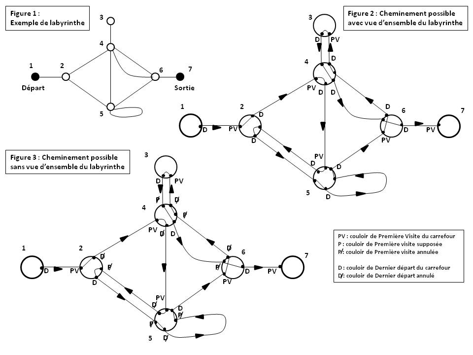
Figure 1 above gives an example of a simple labyrinth made up of 7 crossroads (numbered 1 to 7) including a dead end (crossroads 3), 10 corridors and 4 minimal loops ((55), (464), (2452) and (4564)).
The simplest rule for navigating a labyrinth, called the "hand rule", consists of crossing crossroads and corridors, always leaving the same hand (right or left) placed on the wall. This strategy allows you to never get lost in the labyrinth but does not guarantee finding the exit. Either the traveler possibly discovers one of the exits during his journey, or he automatically returns to his start crossroads.
Thus, on the example of Figure 1, with the right hand rule, a visitor lost at crossroads 5 will go indefinitely in circles in the loop (5245) by entering the corridor (52), and in the loop (5465) by entering the corridor (54).
The "rule of the hand" therefore only applies if the start crossroads corresponds to the entrance to the labyrinth, in which case the traveler is guaranteed to cross the labyrinth without getting lost along the way.
A general rule exists. It allows the lost traveler to definitely escape from the labyrinth when it has an outcome (entrance or exit) and, otherwise, to visit it completely before finding himself at his start crossroads. Two search strategies exist :
- In-depth search, when the traveler is completely lost in the labyrinth. Two different rules were published : rule of Charles-Pierre Trémaux in 1882 [LUC], and rule of Gaston Tarry in 1895 [TAR][TOU][ROS1] which is more general.
- Search by concentric circles (or breadth search), when the traveler knows that he is not too far from the entrance to the labyrinth (less than 3 or 4 crossroads for example). The rule was published by Oystein Ore in 1959 [OYS][WAL].
These three rules (Trémaux, Tarry and Oystein Ore) applie to any flat labyrinth, that is to say spread out on a relatively flat surface, as well as to any three-dimensional labyrinth that may include stairs and rooms with multiple floors.
We now describe Tarry's rule and Oystein's rule, then supplementing them with some general properties of labyrinths (Distinction between crossroads and corridor, and Modeling a labyrinth and shortest path).
B1.2. Tarry : in-depth search
When the traveler is completely lost in the labyrinth, the General Rule of the French mathematician Gaston Tarry is a double rule which is stated as follows :
|
At each crossroads of the labyrinth : Rule no. 1 : Only retake the corridor of first visit to this crossroads as a last resort (Tarry's rule [TAR]). Rule no. 2 : Never take a corridor twice in the same direction (remark from Pierre Tougne [TOU]). Rule no. 1 allows you to escape the labyrinth with certainty. If the labyrinth does not have an outcome (entrance or exit), all crossroads are visited by traveling through each corridor exactly twice before returning to the start crossroads. Rule no. 2 avoids wasting time by retracing paths already taken. This double rule has many practical advantages : - It is easy to remember. - Subject to correctly marking certain particular corridors, it allows you to commute, at any time and without getting lost, between any finish crossroads and any start crossroads, and this without having to go through all the corridors already covered on the way there. This makes it possible in particular to return to a start crossroads (for example to pick up a person left there waiting) then to return to the finish crossroads (for example to bring the person back with you and continue the search together) [PET]. - It allows you to completely clean a labyrinth by passing through all the crossroads without exception. - It allows you to successively cut each of the two sides of each corridor in a hedge labyrinth by passing through all the corridors twice without exception. |
|
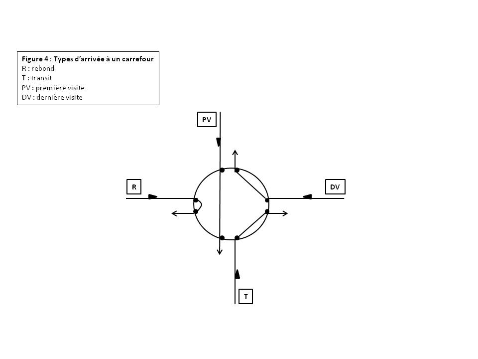
Proof of Tarry's general rule : We will demonstrate that Tarry's rule allows us to visit all the crossroads of the labyrinth when it has no outcome (entrance or exit), which means that we certainly exit the labyrinth otherwise. In the following, we consider that : - A labyrinth is a set of crossroads whose exits are all connected to corridors ; - Any two crossroads are connected by at least one continuous path passing through one or more corridors between crossroads (connected labyrinth) ; - All corridors are two-way ; - The start crossroads is a crossroads already visited by a fictitious arrival corridor. Proposition no. 1 : Crossroads all completely visited (quick demonstration according to [TAR]) : Since the corridors of the labyrinth are all two-way, any crossroads has as many exits as entrances. The traveler is therefore never stuck when visiting or revisiting a crossroads in the labyrinth. Consequently, if the labyrinth has no exit (entrance or exit) and if the rule no. 2 is scrupulously applied, the traveler will eventually stop at the start crossroads. At this moment, all the crossroads of the labyrinth are then necessarily completely visited, with all the corridors traveled exactly twice. Proposition no. 2 : Crossroads all completely visited (complete demonstration by the Author of this Website) : Since the corridors of the labyrinth are all two-way, any crossroads has as many exits as entrances. Consequently (see Figure 4 below), the traveler who enters a crossroads via an arrival corridor (type R or T corridor) necessarily exits via a departure corridor not already taken in this direction (cf rule no. 2). This departure corridor can be the arrival corridor (with R rebound on the crossroads) or any other departure corridor (with T transit through the crossroads). The first arrival at the crossroads (PV corridor) corresponds to the discovery of the crossroads via its corridor of first visit, followed by a departure via any corridor. The last arrival at the crossroads (DV corridor) corresponds to the last visit to the crossroads with a return in the opposite direction to the corridor of first visit (cf rule no. 1). The traveler is therefore never stuck when he visits or revisits a crossroads in the labyrinth. Consequently, if the labyrinth has no outcome (entrance or exit) and if rule no. 2 is scrupulously applied, the traveler will eventually stop at the start crossroads after having visited a certain number of crossroads. Any crossroads visited for the first time is via a corridor traveled from another crossroads necessarily visited for the first time. Consequently, any crossroads visited at least once is on a tree whose trunk is the start crossroads and whose branches are the first visit corridors of each crossroads (see example in Figure 5 below). Suppose that there is on this tree a crossroads whose first visit corridor is never taken in the opposite direction. In this case, the upstream crossroads located on the tree just before this downstream crossroads finds itself in the same situation (see rule no. 1). Step by step, the start crossroads located at the base of the tree (first crossroads visited) also finds itself in the same situation, which is contradictory with the fact that the traveler always ends up returning to the start crossroads. Consequently, if the rule no. 1 has been scrupulously applied at each crossroads, all crossroads in the tree are completely visited. Furthermore, the labyrinth being connected, any crossroads (C) not already visited and connected to a crossroads of the tree at the distance of a corridor will therefore visited, which extends the tree and makes crossroads C completely visited. Step by step, all the crossroads of the labyrinth will therefore be completely visited, with all the corridors of the labyrinth traveled exactly twice (once in the arrival direction and once in the starting direction). On a practical level, the completely visited crossroads of the labyrinth are therefore successively visited in the form of downstream-upstream fallbacks which necessarily end at the start crossroads. On the example of Figure 2 above, if crossroads 7 is not an exit but a simple dead end, the path is as follows : - The route between the departure from crossroads 1 and the arrival at crossroads 7 is given by the succession of corridors (12)(24)(45)(52)(25)(55)(56)(64)(43)(34)(46)(67). See following paragraph. - The route to then return to the crossroads 1 is given by the succession of corridors (76)(64)(46)(65)(55)(54)(42)(21). The fallback corridors are (34) then (76) then (65) then the series (54)(42)(21)), and correspond to the branches of the tree of the corridors of first visit to each crossroads (see Figure 5 below). Conclusion : The traveler therefore visits all the crossroads of the labyrinth when it has no outcome (entrance or exit), which means that one will certainly exit the labyrinth otherwise. |
B1.3. Tarry : course with overview
In the fun case where the traveler has an overview of the labyrinth, the traveler must analyze each crossroads and its adjoining corridors as follows :
A. Just before entering a crossroads, the traveler must mark the Corridor of first Visit to the crossroads (PV) which is the corridor through which the visitor enters the crossroads for the first time. To do this, he creates a PV mark at the right end of the arrival corridor.
B. Just before leaving the crossroads, the traveler must mark the Last departure corridor from the crossroads (D) which is the most recent corridor through which the visitor exits the crossroads. To do this, he creates a D mark at the right entrance to the departure corridor.
Let's see this course on the example of Figure 1.
The crossroads are marked by the numbers 1, 2... 7 where 1 is the start crossroads of the lost traveler and 7 the only outcome of the labyrinth (entrance and exit). The route of a corridor is noted by the number of the start crossroads followed by the number of the end crossroads, for example (24).
Initially, the traveler finds himself lost at crossroads 1 and seeks to reach the exit of the labyrinth (crossroads 7).
Figure 2 above shows a possible course accompanied by the marks created at the end of each arrival corridor (PV or no mark) and at the entrance to each departure corridor (D).
In the case of a dead end (single-exit crossroads), the PV and D marks are not useful since the traveler will never return to this crossroads (see crossroads 3 in Figure 2).
Let's start from the crossroads (1) and take the only possible corridor (12).
At crossroads 2, choose one of the four unexplored corridors, for example (24). At crossroads 4, let's choose, for example, corridor (45). At crossroads 5, let's choose for example corridor (52). Until now, it has been easy to apply the general rule because there was, at each crossroads visited, an unexplored corridor and each crossroads was visited for the first time.
At crossroads 2 (already visited), we cannot take corridor (21) which is the corridor of first visit to the crossroads (cf rule no. 1), nor corridor (24) already taken in this direction (cf rule no. 2). The only option left is to turn back via the corridor (25).
At crossroads 5 (already visited), let's choose for example the right corridor which is in fact a loop (55). Back at crossroads 5, let's choose for example the corridor (56). At crossroads 6, let's choose for example the corridor (64).
At crossroads 6, let's choose, for example, corridor (64).
At crossroads 4 (already visited), by application of rules no. 1 and 2, we can only take one of the two unexplored corridors (43) or (46), or turn back via the other corridor (46).
The first tactic is called "Crazy Ariadne", the second "Sage Ariadne or Trémaux Algorithm". These two tactics are equivalent if we seek to explore the entire labyrinth. The "Crazy Ariadne" tactic is, however, preferable if we are looking for a way out. Let's choose this tactic and take the corridor (43).
At crossroads 3 (dead end), we must turn back via corridor (34).
At crossroads 4 (already visited), let's choose for example the unexplored corridor (46) then, arriving at crossroads 6, the corridor (67) leading to exit 7.
In total, the course between start 1 and exit 7 of the labyrinth is given by the succession of corridors (12)(24)(45)(52)(25)(55)(56)(64)(43)(34)(46)(67).
The corridors of first visit to each crossroads are indicated in bold font.
B1.4. Tarry : course without overview
In the real case where the traveler does not have an overview of the labyrinth, the traveler must stop at each crossroads and go completely around it in order to analyze all the adjoining corridors as follows :
A. Just before entering a cossroads, the traveler must temporarily mark the arrival corridor as the assumed corridor of First Visit to the crossroads. To do this, it creates a P mark at the right end of the arrival corridor. This mark also allows you to go completely around the crossroads, returning calmly to the P mark.
- If the assumption is true (crossroads having no PV mark), the traveler must change the P mark to PV mark in order to be able to apply rule no. 1 during a next visit to the crossroads.
- If the assumption is false (crossroads already having a PV mark), the traveler must cancel the P mark by crossing it out ("P crossed out") in order to return to initial conditions during a next visit to the crossroads.
B. Just before leaving the crossroads, the traveler must mark two particular departure corridors at the right entrance to each corridor. He must first cancel the D mark of the last corridor explored by crossing it out ("D crossed out"). He must then create a D mark on the corridor he is going to take. The "crossed out D" mark is only useful if the traveler plans to commute through the labyrint between an finish crossroads and a start crossroads. Note that, although crossed out, this mark remains a mark of a corridor already explored, therefore eligible for rule no. 2.
Figure 3 above shows the same course as that of Figure 2, accompanied by the marks created at the end of each arrival corridor (P, then PV or P crossed out) and at the entrance to each departure corridor (D crossed out if D exists, then D).
In the case of a dead end (single-exit crossroads), the P, PV and D marks are not useful since the traveler will never return to this crossroads (see crossroads 3 in Figure 3).
In the case where the traveler has nothing to mark the walls of the corridors but where he has small stones (like Tom Thumb), then the marks can be advantageously replaced as follows.
But be careful not to confuse the right entrance and left entrance to each corridor when going around the crossroads !
| Mark | Stone management |
|---|---|
| P | Just before entering a crossroads, place 1 stone at the right end of the arrival corridor. |
| PV | After a complete tour of the crossroads without discovering a pair of stones at the left entrance to a corridor, add 1 stone to the stone placed. |
| P crossed out | During the complete tour of the crossroads with discovery of a pair of stones at the left entrance to a corridor, finish the tour and pick up the stone placed. |
| D crossed out | During the complete tour of the crossroads with discovery of a pair of stones at the right entrance to a corridor, pick up 1 stone out of the 2. |
| D | Just before leaving the crossroads, place 2 stones at the right entrance to the departure corridor. |
B1.5. Tarry : shuttle between two crossroads of the labyrinth
If the traveler has made sure to keep only one D mark at each crossroads (see point B above), he can then commute, at any time and without getting lost, between two crossroads of the labyrinth as following :
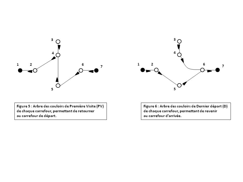
- Returning to a start crossroads (for example to pick up a person left there waiting) then becomes possible and easy. At each crossroads, simply take the corridor marked PV at the left entrance to the corridor in the opposite direction, without generating new marks [PET]. The return path from an finish crossroads to any start crossroads in fact constitutes a tree whose trunk is this start crossroads and whose branches are the corridors marked PV (see Figure 5 below).
Proof : Any crossroads visited the first time is via a corridor traveled from another crossroads necessarily visited the first time. Consequently, any crossroads visited for the first time is on a tree whose trunk is the start crossroads and whose branches are the corridors of first visit to each crossroads.
This tree is called "tree of corridors of first visit to each crossroads" or "tree of crossroads visited the first time".
- Then returning to the finish crossroads (for example to bring the person back with you and continue the search together) also becomes possible and easy. At each crossroads, simply take the corridor marked D at the right entrance to the corridor in the same direction, without generating new marks [PET]. The return path from a start crossroads to any finish crossroads also constitutes a tree whose trunk is this finish crossroads and whose branches are the corridors marked D (see Figure 6 below).
Proof : Any crossroads visited the last time is via a corridor traveled from another crossroads necessarily visited the last time. Consequently, any crossroads visited last time is on a tree whose trunk is the finish crossroads and whose branches are the last departure corridors from each crossroads.
This tree is called "tree of last departure corridors from each crossroads" or "tree of crossroads visited last time".
B1.6. Oystein : search by concentric circles
When the lost traveler knows that he is not too far from the entrance to the labyrinth (less than 2 or 3 crossroads for example), the general rule of the Norwegian mathematician Oystein Ore allows this entrance to be reached by concentric circles from the start crossroads, without the need to explore the labyrinth in depth.
The general rule is then the following [WAL] :
|
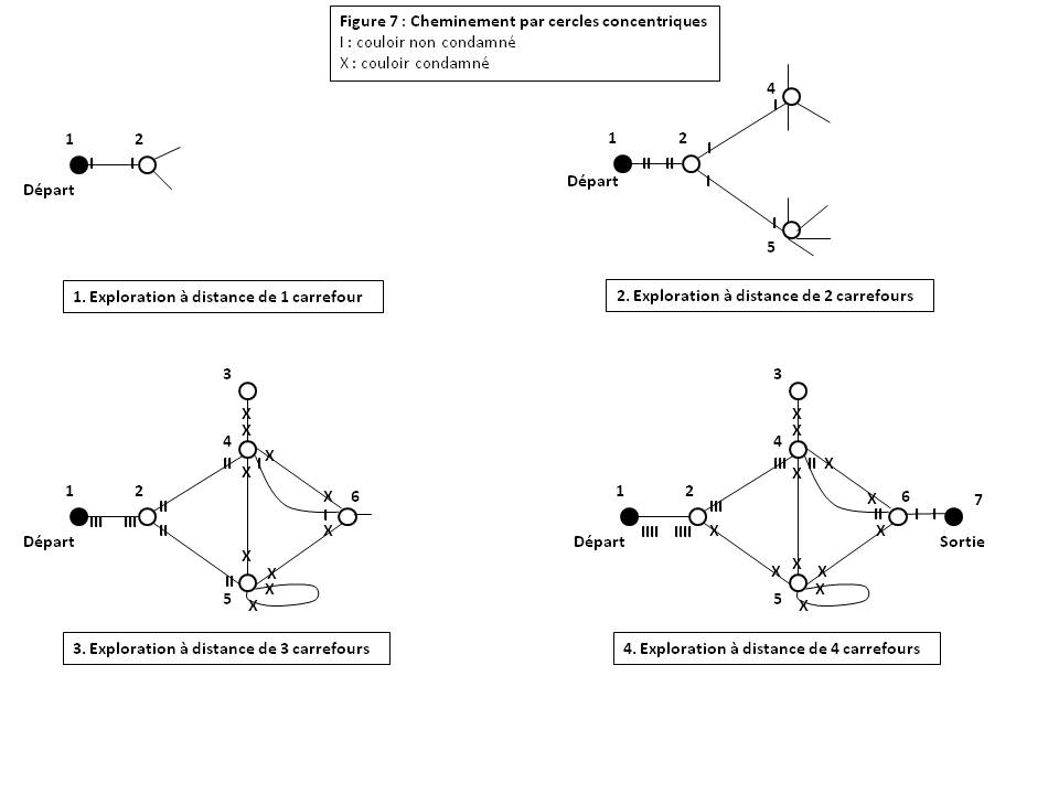
1. From the start crossroads, travel the corridors leading to a distance of 1 crossroads one by one, marking with a line each of the two ends of each corridor traveled. 2. Block both ends of the corridor by changing the marks to a cross in the following four cases : A. the corridor marked with a line is a dead end (corridor (43) in step 3 below) ; B. the corridor marked with a line is a loop connecting two exits from the same crossroads (corridor (55) in step 3 below) ; C. the corridor marked with a line leads to a crossroads already visited (corridors (45), (46) and (56) in step 3 below) ; D. the corridor leads to a crossroads from which all exits are blocked (corridor (25) in step 4 below). 3. Return to the start crossroads following the marks. 4. Repeat the operation by traveling all the non-condemned corridors leading to a distance of 2 crossroads, following the marks, and adding a line at each of the two ends of each corridor during its outward journey. E. The outward and return marks tracking is simple : their number decreases by 1 at each crossroads crossed on the way out and increases by 1 at each crossroads crossed on the way back. 5. Return to the start crossroads following the marks. 6. Repeat the operation as many times as necessary, going at a distance of 3 crossroads, then 4, etc. |
|
Proof of Oystein's general rule : (Complete demonstration by the Author of this Website) Oystein's general rule is to travel the labyrinth by gradually expanding the search in concentric circles passing through the crossroads. The level 0 circle (denoted C0) is the start crossroads. The circle of level n (denoted Cn) whatever n > 0, passes through all the crossroads a crossroads away from the circle Cn - 1. An outward corridor is a corridor connecting a crossroads of the circle Cm to a crossroads of the circle Cm + 1 whatever m ≥ 0. It is always traversed by marking it with an additional line at each end. A return corridor is a corridor connecting a crossroads of the circle Cm + 1 to a crossroads of the circle Cm whatever m ≥ 0. It is always traveled without generating additional marks. Having established these definitions, exploring a new circle Cn + 1 for given n consists of visiting at least once all the crossroads of the circle Cn + 1 using the following strategy : - Reach each crossroads of the Cn circle via the route of outward and/or return corridors following the marks (see law E above), then travel through all the new outward corridors (unmarked and not condemned) connecting this crossroads to the crossroads of the circle Cn + 1. - Return to the start crossroads via the return corridor route following the marks (see law E above). Moreover : - Condemning any corridor connecting two crossroads already visited (see law C above) amounts to removing any loop internal to the labyrinth passing through at least two crossroads (loops (4524), (464) and (5645) in step 3 below), which transforms the labyrinth into a tree whose trunk is the start crossroads and whose foliage is all the uncondemned corridors. - Condemning any dead end (see law A above) amounts to removing any blind corridor connected to the crossroads (corridor (43) in step 3 below), which simplifies the tree by removing the terminale branches. - Condemning any loop connecting two exits from the same crossroads (see law B above) amounts to removing any internal loop at the crossroads (corridor (55) in step 3 below), which simplifies the tree by removing the branches folded on themselves. - Condemning any corridor leading to a crossroads where all exits are condemned (see law D above) amounts to simplifying the tree even further by removing the "dead" branches (corridor (25) in step 4 above). below). The labyrinth finally transforms into a tree whose foliage gradually passes through all the crossroads not yet visited, including inevitably through the exit crossroads from the labyrinth. |
In the fun case where the traveler has an overview of the labyrinth, the general rule applies without difficulty.
Figure 7 below shows a possible course from the start crossroads of the labyrinth in Figure 1, accompanied by the marks created on each corridor traveled (lines or crosses).
The succession of corridors traveled is as follows. Condemned corridors are indicated in bold font.
- Remote exploration of 1 crossroads : (12)(21)
- Remote exploration of 2 crossroads : (12)(24)(42)(25)(52)(21)
- Remote exploration of 3 crossroads : (12)(24)(45)(54)(46)(64)(46)(64)(43)(34)(42)(25)(55)(56)(65)(52)(21)
- Remote exploration of 4 crossroads : (12)(25)(52)(24)(46)(67)
The exit from the labyrinth (also corresponding to the entrance) is found after exploration by concentric circles at a distance of 4 crossroads.
In the real case where the traveler does not have an overview of the labyrinth, the traveler must stop at each crossroads, take a complete tour in order to analyze all the adjoining corridors, then take the return corridor in possibly condemning him. The traveler can then take the wrong corridor when a crossroads has several exits marked with a single line. For example, for crossroads 5 in step 3 below, when taking the return corridor (54), the traveler may mistakenly take the corridor (52) traveled in step 2.
The general rule must therefore be supplemented as follows :
4 bis - Just before entering a crossroads via a new corridor (unmarked and not condemned), when marking the corridor end with a simple line, the traveler must add a different mark (for example P). This particular mark will allow you to calmly take the complete tour of the crossroads and take the return corridor without mistake.
B1.7. Distinction between crossroads and corridor
A labyrinth described in the form of a graph does not present ambiguity between crossroads and corridors, a crossroads being a node of the graph and a corridor an arc connecting two nodes.
But in reality, a crossroads or a corridor is a navigation area that can be complex to analyze at the topological level : more or less vast, more or less narrow area, with the possible presence of niches, shallow dead ends, protusions or small islets. In a crossroads already visited, the traveler may, for example, not find the exact location of an exit or worse, see new corridors appear within the same crossroads. When traveling (in the opposite direction) through a corridor already traveled, the traveler can also, for example, see new crossroads appear within the same corridor.
To avoid any ambiguity, the vocabulary must be rigorously defined as follows :
- A Labyrinth is a set of Crossroads whose Exits are all connected to Corridors.
- A Crossroads is a Navigation area with 1 Exit, 3 Exits, or more than 3 Exits (see example in Figure 8 below). The "1 Exit" case corresponds to a dead end, which is the end of a blind Corridor (crossroads 3 in Figure 1 above), or any single-corridor crossroads that may be a start crossroads (crossroads 1 in Figure 1) or an outcome from the labyrinth (crossroads 7 in Figure 1).
- A Corridor connects two Crossroads by a single Section or by a succession of several consecutive Sections (see example in Figure 8). A Corridor can form a loop when it connects two Exits from the same Crossroads (case of Figure 8).
- A Section is a Navigation area with exactly 2 Exits (see example in Figure 8). A Section is generally empty (without islets) and narrow. It can also be presented in reduced form in length, such as a doorway between two Crossroads.
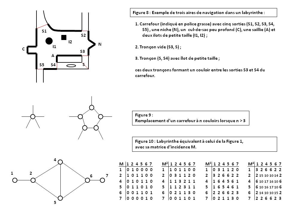
- A Navigation area is a connected space (in one piece) as large as possible, having all its points intervisible or quasi-intervisible, and delimited by one or more Exits. The space may include niches, shallow dead ends, protusions and small islets. Figure 8 below gives an example of three Navigation areas : 1. a Crossroads (indicated in bold font) including five Exits (S1, S2, S3, S4, S5), a niche (N), a shallow dead end (C), a protusion (A) and two small islets (I1, I2)) ; 2. an empty Section (S3, S) ; 3. a Section (S, S4) with a small islet ; these two Sections forming a Corridor between the S3 and S4 Exits of the Crossroads.
- An Exit is the limit of a Crossroads or a Section, beyond which the intervisibility criterion for a Navigation Area is no longer respected.
B1.8. Modeling a labyrinth and shortest path :
When we have an overview of a labyrinth, it can be modeled by an incidence matrix (M) whose rows and columns are the crossroads numbers and each element of the matrix indicates the number of corridors (0, 1, 2, etc.) connecting one crossroads to another [WAL]. Figure 10 above shows an example of a labyrinth and its corresponding incidence matrix.
The incidence matrix also makes it possible to model a labyrinth with one-way corridors [WAL] provided that these corridors do not form a loop connecting two exits from the same crossroads or a loop connecting two crossroads.
For study purposes, any labyrinth can be simplified as follows :
1. Any dead end can be removed by considering that it is integrated (as a shallow dead end) into the crossroads leading to it.
2. Any loop connecting two exits from the same crossroads can be removed by considering that it is integrated (as a small islet) into the crossroads.
3. Any loop connecting two crossroads can be reduced to a single corridor between these crossroads by considering that it is integrated (as a small islet) into this corridor.
4. Any crossroads whose number of corridors is reduced to 2 by one or more of the preceding simplifications can be removed by directly connecting the two corridors.
5. Any crossroads with n corridors such that n > 3 can be replaced by a ring formed by n crossroads with 3 corridors each [STE] on condition of agreeing to violate rule no. 2 in the modified crossroads in order to be able to travel the ring between any two crossroads (see Figure 9 above).
If the traveler knows how to navigate the modified labyrinth, then he or she can also find a path through the original labyrinth by restoring the original crossroads and corridors.
Figure 10 shows the labyrinth equivalent to that of Figure 1 by applying simplifications 1 to 4.
The incidence matrix of a labyrinth makes it possible to find the number of corridors of the shortest path connecting one crossroads to another [WAL].
By multiplying the matrix M by itself (see Figure 10), we obtain a new matrix (M2) whose elements indicate the number of different ways of going from one crossroads to another via a path made up of 2 corridors. By repeating the operation n times, we obtain a matrix (Mn) whose elements indicate the number of different ways of going from one crossroads to another by a path made up of n corridors [WAL].
To find the shortest path connecting one crossroads to another, it is then sufficient to raise the matrix M to a power such that the element corresponding to the connection between these two crossroads becomes non-zero. The power then gives the number of corridors of the shortest path [WAL].
Figure 10 above shows that the shortest path to go from crossroads 1 to crossroads 7 is obtained for n = 4 with 2 possible paths made up of n = 4 corridors.
B1.9. Sources relating to labyrinth
[LUC] Edouard Lucas, Le jeu des labyrinthes, in Récréations mathématiques, tome I (2ème édition, Paris, 1882), chapitre 3, pp. 41-55.
[OYS] Oystein Ore, An excursion into labyrinths, in The Mathematics Teacher, pp. 367-370, Vol. 52, N 5, May 1959.
[PET] Régis Petit, Labyrinthes et arbres, article de la revue "CANAL.N7", journal de l'association des ingénieurs de l'I.E.T.- E.N.S.E.E.I.H, N 33 de septembre 1994.
[ROS1] Pierre Rosensthiel, Les mots du labyrinthe, Revue CoEvoluion. N 11. Hiver 1983.
[ROS2] Pierre Rosensthiel, Labyrintologie mathématique, in Mathématiques et sciences humaines, tome 33 (1971), p.5-32.
[STE] Ian Stewart, Algorithmes labyrinthiques, article de la revue Pour la science, rubrique Visions mathématiques, N 162 d'avril 1991.
[TAR] Gaston Tarry, Le problème des labyrinthes, Nouvelles annales de mathématiques 3e série, tome 14 (1895), p. 187-190.
[TOU] Pierre Tougne, Comment explorer un labyrinthe ?, article de la revue Pour la science, rubrique Jeux mathématiques, N 60 d'octobre 1982, réactualisé dans Pierre Tougne, L'exploration d'un labyrinthe, Dossier Pour la science, Avril/Juin 2008.
[WAL] Jearl Walker, Comment traverser un labyrinthe sans se perdre ni tourner en rond, article de la revue Pour la science, rubrique Expériences d'amateur, février 1987.
Benford's law, or Newcomb-Benford law, or law of abnormal numbers, or law of the first significant digit, shows that in everyday life, the first significant digit of numbers is not equiprobable : the number 1 is more frequent than 2, itself more frequent than 3, etc.
This curiosity is observed in many fields such as the human and social sciences, tables of numerical values, genetics, construction, economics (exchange rates) or even in the street numbers in one's address book [WIK1].
Open the page of a newspaper at random, note all the numbers you find there. Then look at the first significant digit of each number. It is the leftmost digit, which is not zero. Do not take into account either the sign or the place of the decimal point : for example, the first significant digit of the numbers 0.038 3.14159 and -32 is 3.
To your great surprise, you will notice that the digit 1 appears for almost a third of the numbers, the digit 2 approximately once in 6, and that the frequency of appearance decreases until the digit 9 (less than once in 20) [ROU].
B2.1.
Definition :
Benford's law gives the theoretical value (f) of the frequency of appearance of the first significant digit (c) of a measurement result expressed in a given base (b) [WIK1] : fc = logb(1 + 1/c)
We verify that the sum of the frequencies fc is worth : ∑i = 1, (b-1) [logb(1 + 1/i)] = logb(b) = 1
In the decimal system (base b = 10), the law is therefore : fc = log10(1 + 1/c)
For example, the Benfordian probability that a base 10 number begins with the digit c = 1 is as follows : f1 = log10(2) = 30.1 %
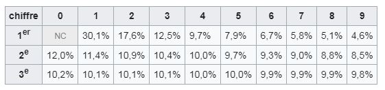
The table above gives the frequency fc in percentage for each value of the first digit c between 1 and 9.
Benford's law remains invariant by changing the number base and also by multiplication by a constant, particularly when changing units.
B2.2.
Application areas :
Benford's law applies all the better when the series of numbers is "rich", with numbers of varied origins (case of a good mixture of any series) and/or relatively well spread over a range covering several orders of magnitude (sizes of cities for example) [ROU][DEL2].
Thus, the house numbers found in an address directory satisfy Benford's law quite well [DEL1]. If a street has 50 numbers, then more than a fifth of the numbers start with a 1 (because of 10, 11, 12... 19). If it has 20 or 200, more than half of the numbers start with a 1. It is therefore normal to find on average more often numbers starting with a 1 than with 9 (and more generally with the digit c than with c + 1) [LED1].
Benford's law does not apply for various cases, including the following [WIK1][DEL1] :
- Numbers drawn at random (the digits c will then all be equally probable).
- Numbers whose first digit is imposed, for example telephone numbers or vehicle registration numbers.
- Restricted scale of possible values, for example the height of individuals in meters (almost all measurements starting with the digit 1) or the selling price of a particular model of new car (the price varies little from one dealer to another) to another).
Benford's law is mainly used to detect tax, financial, accounting and scientific fraud. The principle is as follows : if they regularly extend over several orders of magnitude, the numbers appearing in accounts or statistics must, unless there are special reasons, verify Benford's law. If these are invented numbers, then the forger must have wanted to create as many starting with 1 as with 2, 3, etc., which will contradict Benford's law [DEL2].
In a document containing N numbers, if Nc is the number of times the first significant digit is c, if fc is the frequency of appearance of the digit c according to Benford's law, then we define a test statistic T as follows [AMQ][WIK2] :
T = ∑c = 1, 9 [ (Nc - N fc)2 / (N fc) ] = N ∑c = 1, 9 [ ((Nc/N) - fc)2 / fc ]
For large N, the statistic T then behaves like a variable of the law of X2 at v = (9 - 1) degrees of freedom [AMQ].
By comparing T with the quantile Q of order 95 % of the X2 law with v = 8 degrees of freedom [WIK2], we can conclude that the series of numbers is most certainly faked in the case where T > Q
Benford's law is also used to detect the existence of hidden messages in images (steganography). Two main methods exist [ATO] :
The first method examines the lead digit distribution of the raw contents of the bytes of a suspect image.
The second method examines the distribution of lead digits of quantised discrete cosine transform (DCT) coefficients of the JPEG encoding.
B2.3. Explanation :
Benford's law remains imperfectly explained to this day [DEL1]. The best explanation seems to be this :
We demonstrate mathematically that the sequence of natural integers (1, 2, 3... n) satisfies a "weak" form of Benford's law (in the sense of Cesàro's iterated averages) [DEL1].
This is why it seems legitimate, when the data set is "rich" (see Application areas above), to find statistically in everyday life, series of numbers whose first significant digit is not equiprobable and approximately follows Benford's law.
B2.4. Case of the digits following the first :
1. Case of a block of digits in first position [WIK1] :
The Benfordian probability that a number in base b begins with the digit block (cde) is as follows : fcde = logb(1 + 1/cde)
For example, for the block cde = "314" in base 10, we have : f314 = log10(1 + 1/314) = 0.138 %
Another example, for the block cde = "10" in base 3 (i.e. cde = 3 in base 10), we have : fcde = log3(1 + 1/3) = 26.2 %
2. Case of a digit in position k [WIK1] :
The Benfordian probability that a digit (c) is at a given position (k > 1) in a number in base b is as follows : fc = ∑i = bk-2, (bk-1 - 1) [logb(1 + 1/(i b + c))]
For example, the Benfordian probability in base 10 that the digit c = 0 appears in the second position (k = 2) is : log10(1 + 1/10) + log10(1 + 1/20) + ... + log10(1 + 1/90) = 12.0 %.
This law quickly approaches a uniform law with a value of 10 % for each of the ten digits (see Table above).
B2.5. Case of the sequence of natural integers :
For the sequence of natural integers (1, 2, 3... n), the digits c in base b are only equally distributed (of frequency M = 1/(b - 1))) when n is exactly (b - 1), (b2 - 1)... (bp - 1) for p integer ≥ 1, which almost never happens [CHA].
Otherwise, the frequencies of the first digit c in base b constantly oscillate between two extreme values Msup and Minf taken respectively at nsup and ninf, such that [WIK1][CHA] :
nsup = (c + 1) bp - 1 - 1
ninf = c bp - 1
Msup = ( (bp - 1)/(b - 1) ) / nsup which tends to Msupapp = b/( (c + 1)(b - 1) ) for p = +∞
Minf = ( (bp - 1)/(b - 1) ) / ninf which tends to Minfapp = 1/( c (b - 1) ) for p = +∞
We have the relation : Minf ≤ Minfapp ≤ M ≤ Msupapp < Msup since we always have : 1 ≤ c ≤ b - 1 and b > 1
In base 10 and for p = 1, the value of the couple (Msup, Minf) is
:
(1, 1/9) for the digit 1, obtained in (nsup, ninf) = (1, 9),
(1/5, 1/49) for the digit 5, obtained in (nsup, ninf) = (5, 49),
(1/9, 1/89) for the digit 9, obtained in (nsup, ninf) = (9, 89).
In base 10 and for p = 2, the value of the couple (Msup, Minf) is
:
(11/19, 11/99) for the digit 1, obtained in (nsup, ninf) = (19, 99),
(11/59, 11/499) for the digit 5, obtained in (nsup, ninf) = (59, 499),
(11/99, 11/899) for the digit 9, obtained in (nsup, ninf) = (99, 899).
In base 10 and for p = +∞, the value of the couple (Msupapp, Minfapp) is :
(5/9, 1/9) for the digit 1,
(5/27, 1/45) for the digit 5,
(1/9, 1/81) for the digit 9.
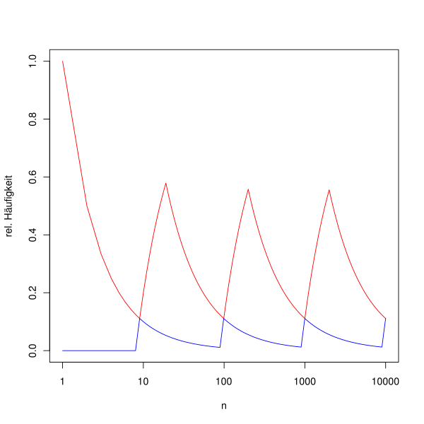
For example, the graph above shows the frequency curve of the first digit 1 (in red) and that of the first digit 9 (in blue) for integers from 1 to 10,000, in logarithmic scale [WIK1].
The sequence fc(n) therefore does not converge and oscillates indefinitely between two extreme values. To smooth these oscillations [DEL1], we take the average sc(n) = (1/n) ∑k = 1, n [fc(k)], called Cesàro average. The new sequence sc(n) still does not converge but varies in a narrower interval.
By repeating this averaging process (tc(n) = (1/n) ∑k = 1, n [sc(k)]), we obtain successive sequences (tc(n), uc(n), etc.) which vary in increasingly narrow intervals and B. Flehinger demonstrated in 1966 that the interval that we obtain by continuing these calculations of averages of averages approaches, to infinity, the expected value of the Benford's law, i.e. logb(1 + 1/c)
Thus, the frequency of integers starting with the digit c satisfies a "weak" form of Benford's law (in the sense of Cesàro's iterated averages), each frequency converging towards the value logb(1 + 1/c)
This convergence in the Cesàro sense makes it possible to converge sequences which were divergent. Known example, the sequence "01010101..." converges to 1/2 in the Cesàro sense.
B2.6. Case of numerical sequences :
Certain remarkable numerical sequences satisfy Benford's law at infinity, that is to say that the proportion of the terms of the sequence up to n, the first digit of which is c, tends towards the value log10(1 + 1 /c) when n tends to infinity.
This is the case of the sequences 2n, nn and (n!), as well as the coefficients of Newton's binomial [DEL1].
It is the same for any sequence rn where r is a positive real such that log10(r) is not a rational number (that is to say a ratio of two integers) [DEL1].
It is also the same for any sequence defined by a recurrence relation of type : u(n) = a1 u(n - 1) + a2 u(n - 2) + ... + ap u(n - p), in particular for the Fibonacci sequence (defined by : u(0) = u(1) = 1 and u(n) = u(n - 1) + u(n - 2)) [DEL1].
B2.7. Sources relating to Benford's law
[AMQ] Association Mathématique du Québec, La loi de Newcomb-Benford ou la loi du premier chiffre significatif.
[ATO] P. Andriotis, T. Tryfonas, G. Oikonomou, T. Spyridopoulos, On Two Different Methods for Steganography Detection in JPEG Images with Benford's Law, NATO Spie conference 2013.
[CHA] Jean-Marie Champeau, Les illusions - La loi de Benford.
[DEL1] Jean-Paul Delahaye, L'étonnante loi de Benford, article de la revue Pour la science, rubrique Logique et calcul, N 351 de janvier 2007.
[DEL2] Jean-Paul Delahaye, Une explication pour la loi de Benford, article de la revue Pour la science, rubrique Logique et calcul, N 489 de juillet 2018.
[ROU] Thierry de la Rue, Gaëlle Chagny, L'incroyable statistique des premiers chiffres, Université de Rouen.
[WIK1] Wikipedia, Loi de Benford.
[WIK2] Wikipedia, Test du X2.
Listed below are the largest crossword puzzles designed without any black squares ("perfect" crossword puzzles)), known in French, English, Italian, Spanish, Latin, Serbian, Croatian,Hungarian, Hebrew, German.
Some crossword puzzles are classic (with different words horizontally and vertically), others are symmetrical (called "word squares" or "magic letter squares").
In both cases, the most "beautiful" crossword puzzles are those for which all words are expressed in the same language and each in the form of a single common noun, that is to say different from a proper noun and without any separator (space, period, hyphen, apostrophe, etc.). They are indicated by the label ***
The records for the largest perfect crossword puzzles in 2024 are as follows :
1. In French :
* Claude Coutanceau (classic 9x9 crossword puzzle)
*** Jean-Charles Meyrignac (classic 9x8 crossword puzzle)
* Michel Laclos (symmetrical 10x10 crossword puzzle)
* Régis Petit (2 symmetrical 10x10 crossword puzzles)
*** Christophe Lecoutre and Sébastien Tabary (symmetrical 9x9 crossword puzzle)
*** Laurent Bartholdi (2 symmetrical 9x9 crossword puzzles)
*** Brice Allenbrand (49 symmetrical 9x9 crossword puzzles)
2. In English :
* Jeff Grant (symmetrical 12x12 crossword puzzle)
* Jeff Grant (symmetrical 11x11 crossword puzzle)
* Rex Gooch (2 symmetrical 11x11 crossword puzzles)
*** Matevz Kovacic (symmetrical 10x10 crossword puzzle)
3. In Italian :
*** Author unknown (symmetrical 8x8 crossword puzzle)
4. In Spanish :
*** Author unknown (symmetrical 8x8 crossword puzzle)
5. In Latin :
*** Eric Tentarelli (2 symmetrical 11x11 crossword puzzles)
6. In Serbian :
* Boris Nazanski (symmetrical 10x10 crossword puzzle)
* Zivota Stankovic (symmetrical 10x10 crossword puzzle)
7. In Croatian :
* Milutin Tepsic (symmetrical 11x11 crossword puzzle)
* Zarka Dokica (symmetrical 11x11 crossword puzzle)
8. In Hungarian :
* Author unknown (classic 9x9 crossword puzzle)
9. In Hebrew :
* Author unknown (classic 10x10 crossword puzzle)
10. In German :
*** Author unknown (symmetrical 7x7 crossword puzzle)
*** Tim (2 symmetrical 7x7 crossword puzzles)
* Tim (symmetrical 7x7 crossword puzzle)
11. In other languages :
Other perfect crossword puzzles are available in otherlanguages (*) but with modest dimensions (8-By-8 and smaller). See [CPT Collection].
(*) Arabic, Armenian, Belarusian, Bulgarian, Chinese, Czech, Danish, Dutch, German, Greek, Hindi, Kazakh, Korean, Lithuanian, Macedonian, Persian (Farsi), Polish, Portuguese, Romanian, Russian, Slovenian, Swedish, Turkish, Ukrainian.
Acknowledgments : The author thanks Jean-Charles Meyrignac for his advice and the provision of some of the sources.
Help us : If you know of any other crossword puzzles that are 8x8 or larger, please Contact us.
B3.1. French crossword puzzles :
Classic crossword puzzles (one 9-By-9 and one 9-By-8 crossword puzzles) :
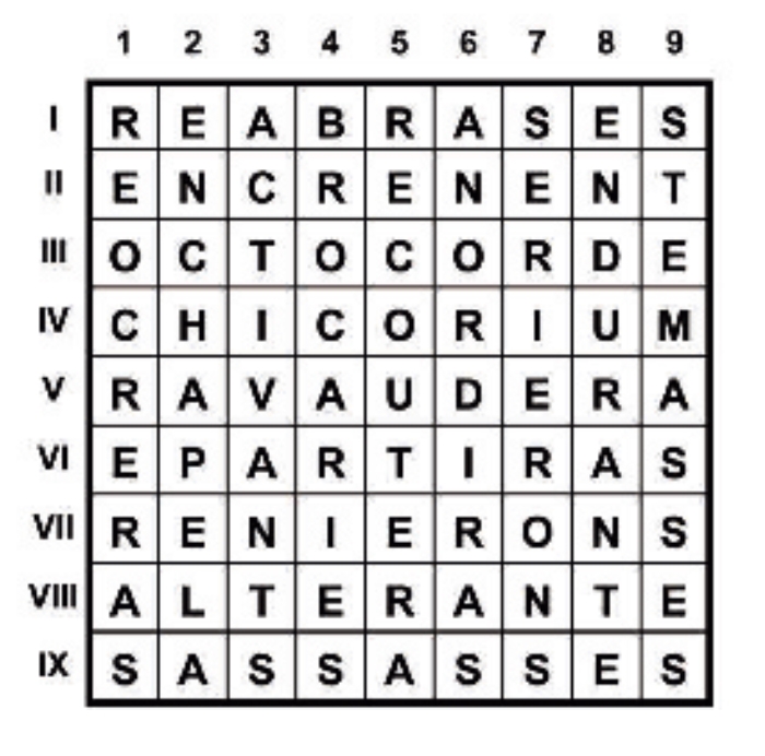
* Figure 1 : 9-By-9 crossword puzzle created in 2010 by Claude Coutanceau [DRI][WIK, Mots croisés].
Horizontally :
REABRASES : du verbe réabraser (abraser à nouveau)
ENCRENENT : du verbe encréner (faire des créneaux)
OCTOCORDE : instrument de musique constitué de 8 cordes à 8 notes conjointes
CHICORIUM :
1. Nom latin utilisé dans les textes botaniques et médicaux pour désigner la chicorée.
2. Erreur d'orthographe en français pour le nom Cichorium, genre botanique relatif aux chicorées. Cette faute se trouve souvent dans les articles culinaires, voire scientifiques.
3. Nom d'une entreprise basée à Pulborough en Angleterre.
RAVAUDERA : du verbe ravauder (raccommoder en couture)
EPARTIRAS : du verbe épartir (épandre)
RENIERONS : du verbe renier (désavouer)
ALTERANTE : de l'adjectif altérant (qui altère)
SASSASSES : du verbe sasser (tamiser)
Vertically :
REOCRERAS : du verbe réocrer (ocrer à nouveau)
ENCHAPELA : du verbe enchapeler (coiffer)
ACTIVANTS : de l'adjectif activant (qui active)
BROCARIES :
1. Ancien écart ou hameau de la commune de Varennes en Dordogne [GOU]
2. Du verbe catalan brocar (deuxième personne du singulier du conditionnel) signifiant percer
RECOUTERA : du verbe recoûter (coûter à nouveau)
ANORDIRAS : du verbe anordir (tourner au nord)
SERIERONS : du verbe sérier (classer)
ENDURANTE : de l'adjectif endurant (qui endure)
STEMASSES : du verbe stemer ou stemmer (faire un stem au ski)
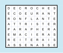
*** Figure 2 : 9-By-8 crossword puzzle created in 2004 by Jean-Charles Meyrignac [ECK, A near-perfect French 9-By-8 word rectangle][WIK, Mots croisés].
Horizontally:
DECROCHES : de l'adjectif décroché
ECOEURANT : de l'adjectif écoeurant
RONFLANTE : de l'adjectif ronflant
ATTRISTER : du verbe attrister
PARAPHERA : du verbe parapher
EMACIERAS : du verbe émacier
REITERAIS : du verbe réitérer
ASSENASSE : du verbe asséner
Vertically:
DERAPERA : du verbe déraper
ECOTAMES : du verbe écôter (enlever la côte des feuilles de certains légumes)
CONTRAIS : du verbe contrer
REFRACTE : du verbe réfracter
OULIPIEN : de l'adjectif oulipien (relatif à l'oeuvre littéraire Oulipo)
CRASHERA : du verbe crasher
HANTERAS : du verbe hanter
ENTERAIS : du verbe enter
STERASSE : du verbe stérer
Word squares (3 10-By-10 and 54 9-By-9 word squares, partial display) :
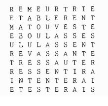
* Figure 1 : 10-By-10 word square published in 1977 in the book "Jeux de lettres, jeux d'esprit" by Michel Laclos [GRA, Ars-magna].
REMEURTRIE : du verbe remeurtrir
ETABLERENT : du verbe établer (mettre à l'étable)
MATOU VESTE : phrase : "matou vesté", le second mot signifiant habillé ou investi en vieux français, ou ennivré en dialecte génevois. Exemple de phrase plausible dans un contexte de littérature médiévale : "Voyez ce fier matou vesté de son pelage noble, qui marche avec l'allure digne d'un seigneur".
EBOULASSES : du verbe ébouler
ULULASSENT : du verbe ululer
REVASSANTE : de l'adjectif rêvassant
TRESSAUTER : du verbe tressauter
RESSENTIRA : du verbe ressentir
INTENTERAI : du verbe intenter
ETESTERAIS : du verbe étester (forme ancienne du verbe étêter)
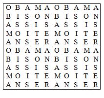
* Figure 2 : 10-By-10 word square created in 2025 by Régis Petit.
This square uses five tautonymous words (each composed of two identical parts) repeated twice.
OBAMA OBAMA :
1. phrase : slogan "Obama ! Obama !" souvent scandé par les partisans lors d'événements en lien avec Barack Obama
2. phrase : titre "Obama Obama" d'un livre néerlandais de Tom-Jan Meeus publié en 2009
3. phrase : titre "Obama Obama" d'une chanson du groupe Millennium en 2008
4. phrase : titre "Obama Obama" d'une chanson de Banjo Beats en 2020
5. phrase : seconde partie du titre de la chanson "Felicidad America (Obama - Obama)" du groupe Boney M., selon deux versions 2009 (anglais et spanglish) adaptées de la version originale 1980 "Felicidad America (Margherita)"
BISON BISON : phrase : nom scientifique du bison d'Amérique
ASSIS-ASSIS : nom : terme médical du domaine de l'aide à la mobilité réduite, désignant le transfert sécurisé d'une personne d'un support assis à un autre support assis (comme d'un fauteuil à un lit en position assise), sans passer par la station debout
MOITE-MOITE : nom : expression familière signifiant moitié-moitié
ANSER ANSER : phrase : nom scientifique de l'oie cendrée
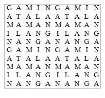
* Figure 3 : 10-By-10 word square created in 2025 by Régis Petit.
This square uses five tautonymous words repeated twice.
PANGA-PANGA : nom : bois dur d'Afrique
ARIUS ARIUS : phrase : nom scientifique du mâchoiron fouet, espèce de poisson-chat
NIAIS ! NIAIS ! ou NIAIS, NIAIS : phrase : répétition apparaissant dans de nombreux textes dramatiques et pièces de foire. Par exemple : "O niais ! niais ! niais !" dans la pièce Othello de Shakespeare (acte V, scène II), traduite par François-Victor Hugo en 1868.
GUILIGUILI : nom : terme familier désignant l'action de chatouiller
ASSIS-ASSIS : nom : terme médical du domaine de l'aide à la mobilité réduite, désignant le transfert sécurisé d'une personne d'un support assis à un autre support assis (comme d'un fauteuil à un lit en position assise), sans passer par la station debout.
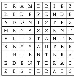
* Figure 4 : 9-By-9 word square published in 1975 in "Pratique des Mots Croisés" by Roger La Ferté and Jacques Capelovici (Que sais-je ? n 1624) [CRU].
TRAMERIEZ : du verbe tramer
REDEPENDE : du verbe redépendre
ADONISTES : botanistes spécialistes des plantes cultivées ou exotiques, dans le contexte de la botanique horticole ancienne
MENASSENT : du verbe mener
EPISTANTE :
1. Adjectif verbal féminin pouvant signifier broyante (mais non officiel en français) et formé sur le verbe épister signifiant broyer ou piler (terme de pharmacie) ;
2. Participe présent (et adjectif verbal) du verbe portugais epistar signifiant broyer ou piler (terme de pharmacie) ;
3. Nom du tableau "Epistante, 2019" peint par Simone Pelligrini, artiste dont l'atelier est à Bologne en Italie.
RESSAUTER : du verbe ressauter
INTENTERA : du verbe intenter
EDENTERAI : du verbe édenter
ZESTERAIS : du verbe zester
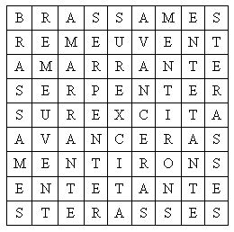
* Figure 5 : 9-By-9 word square published in 1977 in the book of Guy Brouty "Les Mots Croisés, toute une histoire" (Hachette) [CRU]. See [CHA].
BRASSAMES : du verbe brasser
REMEUVENT : du verbe remouvoir
AMARRANTE :
1. Erreur d'orthographe courante pour le nom amarante, plante relative au genre botanique Amaranthus. Cette faute se trouve souvent dans les articles culinaires.
2. Adjectif verbal féminin pouvant signifier captivante, attachante ou qui amarre (mais non officiel en français) et formé sur le verbe amarrer ;
3. Personnage "Amarrante" de la série d'albums pour enfants "Les Florafées" créée par H.F. Diané ;
4. Deux villas de vacances "Borgo Amarrante" et "Molino di Amarrante" situées à Montaione en Toscane (Italie) ;
5. Participe présent du vieux verbe italien amarrare signifiant amarrer.
SERPENTER : du verbe serpenter
SUREXCITA : du verbe surexciter
AVANCERAS : du verbe avancer
MENTIRONS : du verbe mentir
ENTETANTE : de l'adjectif entêtant
STERASSES : du verbe stérer
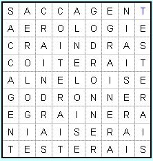
*** Figure 6 : 9-By-9 word square produced in 2007 by Christophe Lecoutre and Sébastien Tabary [LGD, Les Carrés symétriques-4].
SACCAGENT : du verbe saccager
AEROLOGIE : du nom aérologie
CRAINDRAS : du verbe craindre
COITERAIT : du verbe coïter
ALNELOISE : de l'adjectif alnélois (relatif aux habitants de la commune d'Auneau en Eure-et-Loir)
GODRONNER : du verbe godronner (border de godrons)
EGRAINERA : du verbe égrainer
NIAISERAI : du verbe niaiser
TESTERAIS : du verbe tester
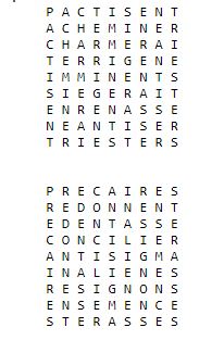
*** Figure 7 : 9-By-9 word square produced in 1996 by Laurent Bartholdi [WIK, Carré magique][WIK, Mots croisés] and communicated by Patrick Jenty [LGD, Symmetrical Squares-4].
PACTISENT : du verbe pactiser
ACHEMINER : du verbe acheminer
CHARMERAI : du verbe charmer
TERRIGENE : de l'adjectif terrigène (qui provient de l'érosion des terres)
IMMINENTS : de l'adjectif imminent
SIEGERAIT : du verbe siéger
ENRENASSE : du verbe enrêner (mettre les rênes)
NEANTISER : du verbe néantiser
TRIESTERS : composés organiques possédant trois fois la fonction ester
*** Figure 8 : 9-By-9 word square produced in 1996 by Laurent Bartholdi [WIK, Carré magique][WIK, Mots croisés] and communicated by Patrick Jenty [LGD, Symmetrical Squares-4].
PRECAIRES : de l'adjectif précaire
REDONNENT : du verbe redonner
EDENTASSE : du verbe édenter
CONCILIER : du verbe concilier
ANTISIGMA : lettre en forme de sigma renversé
INALIENES : de l'adjectif inaliéné
RESIGNONS : du verbe résigner
ENSEMENCE : du verbe ensemencer
STERASSES : du verbe stérer
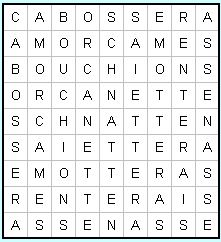
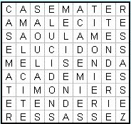
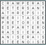
*** Figures 9, 10 and 11 : 6 9-By-9 word squares (with alternatives) produced in 2007 by Brice Allenbrand [LGD, Les Carrés symétriques-4][ALL].
Grille CABOSSERA
Grille CASEMATER : Trois variantes sont possibles en remplaçant Z par E, R ou S dans RESSASSEZ
Grille CRAMPERAS
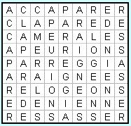
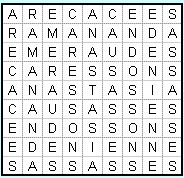
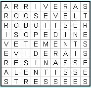
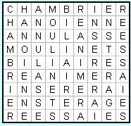
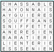
*** Figures 12 then 13 to 24 : 43 9-By-9 word squares (with alternatives) produced in 2008 by Brice Allenbrand [LGD, Les Carrés symétriques-3][LGD, Les Carrés symétriques-2][LGD, Les Carrés symétriques-1].
Grille ACCAPARER : Trois variantes sont possibles en remplaçant le R final par E, S ou Z dans RESSASSER
Grille ARECACEES
Grille ARRIVERAS
Grille CHAMBRIER
Grille CHASSABLE
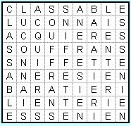
Grille CLASSABLE
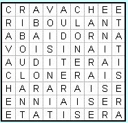
Grille CRAVACHEE
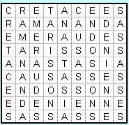
Grille CRETACEES
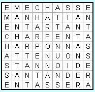
Grille EMECHASSE : Cinq variantes sont possibles en remplaçant le premier T par C dans ENTARTANT, et/ou U par D ou T dans ATTENUONS
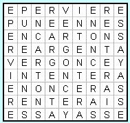
Grille EPERVIERE : Cinq variantes sont possibles en remplaçant C par T dans ENCARTONS, ou (C par S dans ENCARTONS, et premier N par S dans PUNEENNES), ou N par I dans ESSARTONS (en ligne horizontale et/ou verticale)
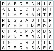
Grille RAFRECHIS : Deux variantes sont possibles en remplaçant le deuxième T par R ou S dans INTERDITE
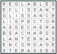
Grille REGLABLES
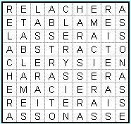
Grille RELACHERA : Quinze variantes sont possibles en remplaçant L par M dans RELACHERA (en ligne horizontale et/ou verticale), et/ou troisième S par I dans ASSONASSE (en ligne horizontale et/ou verticale)
B3.2. English crossword puzzles :
Word squares (1 12-By-12, 3 11-By-11 and 164 10-By-10 word squares, partial display) :
* Figure 1 : 12-By-12 word square produced in 2009 by Jeff Grant.
This square uses six tautonymous words repeated twice [GRA, Some of my favorite squares].
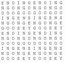
ENDING-ENDING : noun : the conclusion of the last part of a movie, play, book, etc.
NGONGO-NGONGO : proper noun :
1. Locality, Bengo Province, Angola, 8 1'S, 14 32'E
2. Stream, Sangha region, Congo, 1 33'N, 15 41'E
DOOGOO-DOOGOO : noun : variant of dugu-dugu, the sex act, or to have sex, in modern Jamaican English slang.
INGENS INGENS : phrase : Megascops ingens ingens, subspecies of South American Rufescent Screech-Owl.
NGONGENGONGE : noun : clipped person in New Zealand Maori.
GOOSEY-GOOSEY : noun : variant of goosey, a foolish person, a simpleton, for example in the well-known English nursery rhyme "Goosey-Goosey Gander".
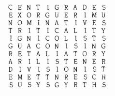
* Figure 2 : 11-By-11 word square produced in 1987 by Jeff Grant [GRA, Quasi eleven-squares].
This square includes proper.
CENTIGRADES : noun : thermometers using the centigrade scale.
EX-ORGUE RIMU : phrase : a nonce-term describing rimu wood formerly used in an orgue. 'Orgue' is defined as 'any of a number of long, thick timbers, pointed and shod with iron, formerly suspended over, or in the vaulted passage behind, a gateway, to be let down in case of attack; also, these pieces collectively'.
NOMINATIVES : noun : words in the nominative case, in grammar.
TRITICALITY : noun : triteness.
IGNICOLISTS : noun : worshippers of fire.
GUACONISING : noun : variant form of 'guaconizing', treating with guano.
RETALIATORY : adj. : tending to, involving, or of the nature of, retaliation.
ARI LISTENER : phrase : a listening person from the small community of Ari, Indiana. For example, a conversation between a resident of Ari, and one from Fort Wayne (12 miles away) could involve a Fort Wayne speaker and an 'Ari listener'.
DIVISIONIST : noun : an advocate of the painting method known as divisionism.
EMETT 'N RESCH : phrase : Emett and Resch are both surnames Iisted in the 1983 Melbourne, Australia, telephone directory. The form 'n is shown in Webster's Third Edition as a shortening of 'and'.
SUSY'S GYRTHS : phrase : a nonce-term describing the refuges of someone named Susy, back in olden times. 'Susy' is shown in What to Narne the Baby, by Evelyn Wells, as a diminutive of 'Susan'. 'Gyrth' is an obsolete form of 'grith', a refuge or sanctuary.
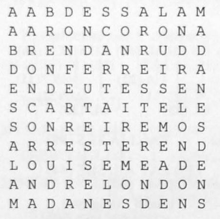
* Figure 3 : 11-By-11 word square produced in 2004 by Rex Gooch [GOO, The eleven-square - Take one].
This square includes foreign terms and double names associated with American first and last names.
AABD ES SALAM : proper noun : Aabd es Salam, Syria, 36 45'N, 40 17'E
AARON CORONA : proper noun : Aaron Corona is the U.S. Marine Corps Lance Cpl., a protective security detail team member with 3rd Battalion, 7th Marine Regiment.
BRENDAN RUDD : proper noun : Brendan Rudd lives in Star, Idaho.
DON FERREIRA : proper noun : Don Ferreira lives in Brentwood, California, or in Klamath Falls, Oregon.
ENDEUTESSEN : conjugated verb : from Catalan verb endeutar-se (third person plural of the imperfect subjunctive) meaning to get into debt.
SCARTAITELE : conjugated verb : from Romanian verb a scartai (second person singular of the imperfect indicative) meaning to creak.
SONREIREMOS : conjugated verb : from Spanish verb sonreir (first person plural of the futur indicative) meaning to smile.
ARRESTEREND : conjugated verb : from Deutsch verb arresteren (present participle) meaning to arrest.
LOUISE MEADE : proper noun : Louise Meade lives in Lebanon, Indiana, or in Xichita, Kansas.
ANDRE LONDON : proper noun : Andre London lives in Douglasville, Georgia.
MADANE'S DENS : phrase : Madane's dens is a manufactured phrase. Madane is a locality in Oio region, Guinea-Bissau, 12 11'N, 15 19'W
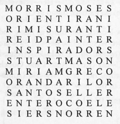
* Figure 4 : 11-By-11 word square produced in 2005 by Rex Gooch [GOO, The eleven-square - Take two][GRA, Some of my favorite squares].
This square includes foreign terms and double names associated with first and last names.
MORRIS MOSES : proper noun : Sir Morris Moses (1762-1830), later called Captain Ximenes. An alternative squares uses Norris-Moses, surname of American representational artist Dorothy NORRIS-MOSES [GRA, Some of my favorite squares].
ORIENTIRANI : verbal adj. : oriented in Slovenian.
RIMISURANTI : conjugated verb : from Italian verb rimisurare (present participle) meaning to remeasure.
REID PAINTER : proper noun : Reid Painter, a pupil recorded on the 5th grade Elementary "A/B" Honor Rolls for October 2003 and January 2004 in North Chatham School, Chatham County, North Carolina.
INSPIRADORS : noun : inspirators in Catalan.
STUART MASON : proper noun : Dr Stuart Mason, English endocrinologist (1919-2003). A second alternative squares uses Stuart Mahon (a redident of Dublin, Ireland) and Santo Helier (a Spanish version of the name of the 6th century ascetic hermit (St. Heller), and also the capital of Jersey in the Channel Islands, which is named after him) [GRA, Some of my favorite squares].
MIRIAM GRECO : proper noun : Miriam Greco and her husband David sold a property at 343 Barclay St, Burlington County, Philadelphia, around January 2004.
ORANDARILOR : noun : from Romanian noun orandar (genitive or dative plural form) meaning someone who owns an inn.
SANTOS ELLER : double proper noun : a Brazilian double surname. A Brazilian website devoted to the genealogy of the Eller family records "Maria dos SANTOS ELLER (born 3 June 1932)".
ENTEROCOELE : noun : the body cavity formed from an outpocketing of the archenteron (a primitive digestive cavity), especially typical of echinoderms and chordates.
SIERSNORREN : proper noun : a contrived Dutch meaning something like ostentatiously-decorated moustaches, formed by combinig sier (decorative or ornamental) with snorren (moustaches).
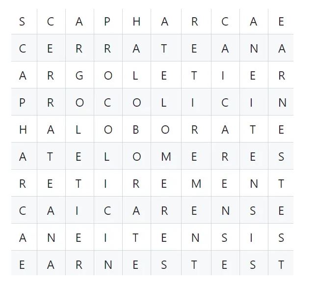
*** Figure 5 : 10-By-10 word square produced in 2023 by Matevz Kovacic, Sloveny [KOV][CAM].
All ten words are unique common nouns.
SCAPHARCAE : adj. : specific epithet of bacterium name Ornithinibacillus scapharcae
CERRATEANA : adj. : specific epithet of plant name Pitcairnia cerreteana
ARGOLETIER : noon : a light mouted soldier ; a mounted bowman
PROCOLICIN : noon : a propeptide form of colicin
HALOBORATE : noon : a type of inorganic compound
ATELOMERES : adj. : specific epithet of moth name Ectropis atelomeres
RETIREMENT : noon : withdrawal from one's position or occupation or form active working live
CAICARENSE : adj. : specific epithet of plant name Machaerium caicarense
ANEITENSIS : adj. : specific epithet of tree fern name Alsophila aneitensis
EARNESTEST : adj. : superlative form of earnest
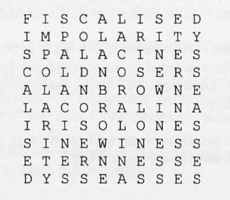
* Figure 6 : 10-By-10 word square produced in 2006 by Jeff Grant [GRA, FISCALISED ten-square revisited][GRA, The best ten-squares].
FISCALISED : verbal adj. : variant of fiscalized
IMPOLARITY : noun : absence of polarity
SPALACINES : noun : blind mole-rats of the subfamily Spalacinae
COLDNOSERS : noun : slang for hunting dogs that follow cold trails
ALAN BROWNE : proper noun : an American bank consultant (1908-88), in Who's Who in America, 45th Ed., 1988-89.
LA CORALINA : proper noun : locality located in the town of Candelaria, Artemisa province, Western Cuba, 22 45'N, 82 57'W
IRISOLONES : noun : colourless estrogenic compounds derived from certain irises
SINEWINESS : noun : state or quality of being sinewy ; firm strength
ETERNNESSE : noun : variant of eternness, eternity
DYSSEASSES : noun : 16th century forms of the noun diseases
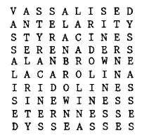
* Figure 7 : 10-By-10 word square produced in 1995 by Jeff Grant [GRA, A spooner-assisted ten-square].
VASSALISED : verbal adj. : subdued, subjugated
ANTELARITY : noun : a blend of antelation (preference, precedence) and priority attributed to the Reverend William Spooner when mixing up the words of 17th-century Spanish scholar James Mabber : "Alleging the antelarity of time, and priotion of his debt".
STYRACINES : noun : white crystalline substances obtained from storax and balsam of Peru
SERENADERS : noun : people who serenade, entertain with music
ALAN BROWNE : proper noun : an American bank consultant (1908-88), in Who's Who in America, 45th Ed., 1988-89.
LA CAROLINA : proper noun : town located in the Jaén province, Spain, 38 16'N, 3 37'W
IRIDOLINES : noun : oily liquid compounds derived from coal-tar
SINEWINESS : noun : state or quality of being sinewy ; firm strength
ETERNNESS : noun : variant of eternness, eternity
DYSSEASSES : noun : 16th century forms of the noun diseases
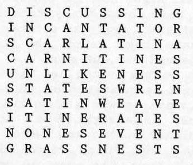
* Figure 8 : 10-By-10 word square produced in 1998 by Ted Clarke [CLA, A new Wordsworth word square][LAN].
DISCUSSING : verbal noun : talking
INCANTATOR : noun : one who uses incantation
SCARLATINA : noun : scarlet fever
CARNITINES : noun : enzymes that transport activated long-chain fatty acids across the mitochondrial membrane
UNLIKENESS : adj. : of little ressemblance
STATE'S WREN : phrase : little bird on flag of some US states (especially South Carolina)
SATIN WEAVE : phrase : silk-like cloth.
ITINERATES : conjugated verb : wanders aimlessly
NONES EVENT : phrase : plausible festival of the ancient Romans
GRASS NESTS : phrase : nests made by weaver birds for example
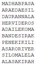
* Figure 9 : 10-By-10 word square produced in 2008 by Martin Laeuter [cf email of September 8, 2024 from Jean-Charles Meyrignac to Régis Petit].
MADHAB PASA : proper noun : Madhab Pasa, village, babuganj upazila region, Bangladesh, 22 46'N, 90 17'E
ARAEDAESIL : proper noun : Araedaesil, town, Chungcheongnam-do region, South Korea, 36 49'N, 126 58'E
DAURAN NALA : proper noun : Dauran Nala, intermittent stream, Balochistan, Pakistan, 30 20'N, 67 23'E
HERVIDEROS : proper noun : Los Hervideros, tourist site, Lanzarote island, Canary Islands, Spain, 28 57'N, 13 50'O
ADAILE-KOMA : proper noun : Adaïlé-Koma, mountain, Djibouti, 11 29'N, 42 33'E
BAND-E SIRAK : proper noun : Band-e Sirak, mountain, Wilayat-e Ghor Province, Afghanistan, 33 27'N, 65 7'E. An alternative square uses Band-e Zirak
PENE-KIKILI : proper noun : Pene-Kikili, town, Maniema Province, Congo-Kinshasa, 4 36'S, 26 20'E
ASARO RIVER : proper noun : Asaro River, river, Eastern Highlands Province, Papua New Guinea, 6 22'S, 145 12'E
SILOMALELA : proper noun : Silomalela, village, Nias island, North Sumatra Province, Indonesia, 1 6'N, 97 39'E
AL'ASAKIRAH : proper noun :
1. Al'Asakirah, village, Dhamar Governorate, Yemen, 14 33'N, 44 40'E
2. Al'Asakirah, village, Dhi Qar region, Irak, 31 0'N, 46 21'E
3. Al'Asakirah, village, Bani Suwayf region, Egypt, 28 55'N, 30 53'E
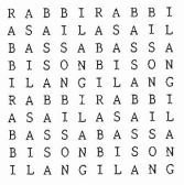
* Figure 10 : 10-By-10 word square produced in 1973 by Dmitri Borgmann.
This square uses five tautonymous words repeated twice [BOR, A new 100-letter word square][GRA, Ars-magna].
RABBI, RABBI : phrase : included in the verse "And greetings in the markets, and to be called of men, Rabbi, Rabbi" in "Gospel According to Saint Matthew", Chapter 23, Verse 7 (cf "The New Testament and the Book of Psalms", King James Version, published by the American Bible Society (New York, 1972)).
A SAIL ! A SAIL ! : phrase : included in the poetic quotation "I bit my arm, I sucked the blood, And cried, A sail ! a sail !" of Taylor Coleridge in "The Rime of the Ancient Mariner", Part III, Stanza 4 (cf "Familiar Quotations" by John Bartlett, 14th Edition, Revised and Enlarged, published by Little, Brown and Company (Boston and Toronto, 1968)).
BASSA-BASSA : noun : general confusion, noise, and, in some cases, exchange of blows (cf "Notes for a Glossary of Words and Phrases of Barbadian Dialect" by Frank A. Collymore, published by Advocate Company (Bridgetown, Barbados, 1970)).
BISON BISON : phrase : Bison bison, scientific (genus + species) name for the bison, a hoofed animal of western North America (cf "The American Heritage Dictionary of the English Language" edited by William Morris, published jointly by American Heritage Publishing Company, Inc., and Houghton Mifflin Company (Boston, New York, Atlanta, Geneva, Illionis, Dallas, Palo Alto, California, 1971)).
ILANG-ILANG : noun : variant spelling of ylang-ylang, a tree native to the Phillippines, Java and India (cf "The World Book Dictionary" edited by Clarerce L. Barnhart, a Thorndike-Barnhart Dictonary published exclusively for Field Enterprises Educational Corporation (Chicago, London, Rome, Stockholm, Sydney, Toronto, 1968)).
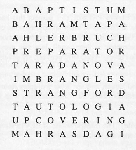
* Figure 11 : 10-By-10 word square produced in 2002 by Rex Gooch [GOO, An A to Z of ten-squares][GOO, My first ten-square].
ABAPTISTUM : noun : abaptiston (cone-shaped trephine)
BAHRAMTAPA : proper noun : in Azerbaijan, 39 44'N, 47 57'E
AHLERBRUCH : proper noun : in Germany, 52 12'N, 8 29'E
PREPARATOR : noun : a person who prepares
TARADANOVA : proper noun : in Russia, 54 45'N, 86 41'E. An alternative square uses Tarakanova, 55 21'N, 38 57'E, also in Russia.
IMBRANGLES : conjugated verb : old form of embrangles
STRANGFORD : proper noun : Strangford :
1. Village, Herefordshire, England, 51 57'N, 2 37'W
2. Farmstead, New Zealand, 43 16'S, 172 06'E
TAUTOLOGIA : noun : Late Latin (or Greek), whence tautology
UPCOVERING : verbal noun : old form of up covering
MAHRAS DAGI : proper noun : Mahras Dagi in Turkey, 36 43'N, 33 17'E
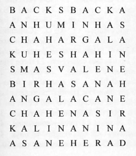
* Figure 12 : 10-By-10 word square produced in 2003 by Rex Gooch [GOO, Ten-squares with place names].
BACKSBACKA : proper noun : Backsbacka, Finland, 63 27'N, 23 07'E
ANHUMINAS : proper noun : Ribeirao Anhuminhas, Brazil, 22 53'S, 50 50'W
CHAHARGAL'A : proper noun : Chahargal'a-i-Wazirabad, Afghanistan, 34 33'N, 69 09'E
KUH-E SHAHIN : proper noun : Kuh-e Shahin, Iran, 35 24'N, 46 32'E
SMASVALENE : proper noun : Smasvalene, Norway, 60 58'N, 4 38'E
BI'R HASANAH : proper noun : Bi'r Hasanah, Finland, 30 27'N, 33 46'E
ANGALACANE : proper noun : Angalacane, Mozambique, 22 28'S, 31 31'E
CHAH-E NASIR : proper noun : Chah-e Nasir, Iran, 27 43'N, 58 01'E
KALINANINA : proper noun : Kalinanina, Zambia, 14 23'S, 24 44'E
ASANE HERAD : proper noun : Asane Herad, Norway, 60 28'N, 5 25'E
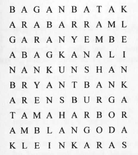
* Figure 13 : 10-By-10 word square produced in 2003 by Rex Gooch [GOO, Ten-squares with place names].
BAGANBATAK : proper noun : Baganbatak, Columbia, 3 12'N, 99 40'E
'ARAB AR RAML : proper noun : 'Arab ar Raml, Egypt, 30 31'N, 31 12'E
GARANYEMBE : proper noun : Garanyembe, Zambia, 14 25'S, 26 56'E
ABAG KANALI : proper noun : Abag Kanali, Azerbaijan, 39 11'N,48 36'E
NANKUNSHAN : proper noun : Nankunshan, China, 23 38'N, 113 53'E. An alternative square uses Nankan Shan, Taiwan, 25 04'N, 121 18'E
BRYANT BANK : proper noun : Bryant Bank, an undersea feature, 28 01'N, 92 28'W
ARENSBURGA : proper noun : Arensburga, Estonia, 58 14'N, 22 30'E
TAMA HARBOR : proper noun : Tama Harbor, Japan, 34 28'N, 133 56'E
AMBLANGODA : proper noun : Amblangoda, Sri Lanka, 7 00'N, 81 11'E
KLEIN-KARAS : proper noun : Klein-Karas, Namibia, railroad siding, 27 34'S, 18 06'E
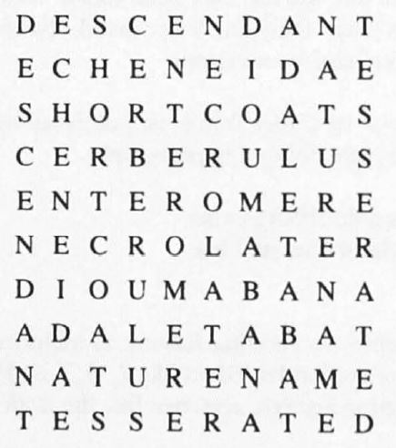
* Figure 14 : 10-By-10 word square produced in 2002 by Rex Gooch [GRA, The best ten-squares][GOO, Some superior ten-squares][CAM].
DESCENDANT : noun : one descended from an ancestor ; issue, offspring
ECHENEIDAE : noun : the remora family of fishes
SHORTCOATS : noun : people wearing short coats
CERBERULUS : adj. : specific epithet of ant name Camponotus cerberulus
ENTEROMERE : noun : any segment of the embryonic alimentary tract
NECROLATER : noun : someone who worships the dead or dead bodies
DIOUMABANA : proper noun : a populated place in eastern Guinea, West Africa, 11 16'N, 9 08'W
ADALETABAT : proper noun : a populated place in the Mus province, eastern Turkey, 38 58'N, 42 42'W
NATURE-NAME : noun : a toponym (place name) embodying an allusion to a natural occurrence or geographical feature
TESSERATED : verbal adj. : rare variant of tessellated, composed of small blocks of variously coloured material arranged to form a pattern
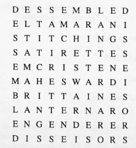
* Figure 15 : 10-By-10 word square produced in 2002 by Rex Gooch [GOO, Some superior ten-squares].
DESSEMBLED : verbal adj. : come from the old French verb dissembler meaning to dissemble
EL-TAMARANI : proper noun : Wadi el-Tamarani, Egypt, 29 52'N, 34 32'E
STITCHINGS : verbal noun : activities of sewing individual threads in something
SATIRETTES : noun : small satires
EMCRISTENE : noun : old form of fellow Christian. An alternative square uses emcrystene
MAHESWARDI : proper noun : Nagar Maheswardi, Bangladesh, 24 04'N, 90 42'E,
BRITTAINES : noun : old form of Britons
LANTERNARO : noun : lantern maker or seller (of Italian origin)
ENGENDERER : noun : producer, causer or bringer
DISSEISORS : noun : persons who wrongfully dispossess
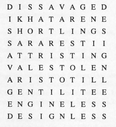
* Figure 16 : 10-By-10 word square produced in 2002 by Rex Gooch [GOO, Some superior ten-squares].
The ten words are all without separators (space, period, hyphen or apostrophe).
DISSAVAGED : verbal adj. : civilized
IKHATARENE : proper noun : Ikhatarene, Morocco, 33 17'N, 4 44'W
SHORTLINGS : noun : short or small persons
SARARESTII : proper noun : Sararestii, Romania, 44 56'N, 24 52'E
ATTRISTING : verbal noun : saddening
VALESTOLEN : proper noun : Valestolen, Norway, 60 49'N, 5 32'E
ARISTOTILL : proper noun : medieval form of the proper noun Aristotle
GENTILITEE : noun : medieval form of the noun gentility
ENGINELESS : adj. : without an engine
DESIGNLESS : adj. : being without a design
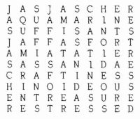
* Figure 17 : 10-By-10 word square produced in 1990 by G.H. Ropes [ROP, Further struggles with a ten-square].
JAS J. ASCHER : proper noun : name of James J. Ascher found in a Kansas City telephone directory
AQUAMARINE : noun : transparent blue-green gemstone
SUFFISANTS : noun : citation-word plural for the obsolete adjective suffisant meaning sufficient
JAFFA'S FORT : phrase : old military structure located in Jaffa, Palestine
AMIATA TIER : phrase : Amiata is a mountain in the Apennine range in central Italy, part of a long chain which could plausibly be named the Amiata Tier
SASSANIDAE : proper noun : members of the native dynasty that built and ruled an empire in Persia from 224 to 636
CRAFTINESS : noun : cunning
HINOIDEOUS : adj. : with veins proceeding from the midrib parallel and unbranched (venation of the leaves)
ENTREASURE : verb : to lay up in or as in a treasury
RESTRESSED : adj. : stressed again
* 5 other 10-By-10 word squares produced in 1990 and 2002 by Jeff Grant.
These squares include foreign terms and double names associated with American first and last names. See [GRA, A modified ten-square][GRA, In search of the ten-square].
1 ASTRALISED square
1 DISTALISED square
1 DORAASCHER square
1 INCAPABLER square
1 MISSATICAL square
* 35 other 10-By-10 word squares (with alternatives) produced in 2003 by Rex Gooch.
These squares begin with each letter of the alphabet including separators (space, period, hyphen or apostrophe). See [GOO, An A to Z of ten-squares].
1 BANPAKKHEN square
1 CILASTATIN square
2 EPICOPARI squares
1 FABODTRASK square
1 GATSCHAPAR square
2 HARADSMALA squares
1 IMPRESSUS square
1 JASTREBACA square
1 KACHIKAMAR square
1 LATCHESNES square
1 MACABABALO square
1 MAIDENPAPS square
1 MALENESSES square
1 NISISASPRO square
1 OCHIRIKROM square
1 OMIMICREEK square
1 PARADISIAL square
2 PASSAGE-BED squares
1 QALA'-I-NAMAK square
1 RESISTLESS square
2 SPASMODISM squares
1 TANAMALALA square
1 UNTUNNELED square
1 VALEAHOGEA square
1 WADIEL'EISH square
1 WADIGHABAT square
1 WALSHOUTEM square
1 XOMBANTANG square
2 YATTAWATTE squares
1 ZUSAMMFALL square
* 108 other 10-By-10 word squares (with alternatives) produced in 2003 by Rex Gooch.
These squares use five tautonymous or quasi-tautonymous words, repeated twice. See [GOO, Quarter ten-squares].
10 ABANGABANG squares
12 ALANGALANG squares
18 ANTINANTIN squares
5 CLANGCLANG squares
1 HANGIHANGI square
1 ILANGILANG square
27 INGITINGIT squares
1 MANGIMANGI square
2 ORANGOTANG squares
1 ORANGUTANG square
1 RENGARENGA square
1 SANGASANGA square
1 SANGISANGI square
1 TANGITANGI square
21 UNGASUNGAS squares
1 URANGUTANG square
1 WALLAWALLA square
1 WANGIWANGI square
1 WHANGWHANG square
1 YLANGYLANG square
* 3 other 10-By-10 word squares (with alternatives) produced in 2004 by Rex Gooch.
These squares include separators (space, period, hyphen or apostrophe). See [GOO, Hunting the ten-square].
2 NOSTOCACEA square
1 UORESPECHE square
B3.3. Italien crossword puzzles :
Word squares (1 8-By-8 word square) :
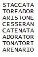
*** 1 8-By-8 square published in 1965 by Dmitri Borgmann [BOR, Language on Vacation, p.198].
STACCATA : verbal adj. : detached
TOREADOR : noun : bullfighter ; the more usual Italian word, however, is "toreadore".
ARISTONE : noun : kind of hand organ
CESSERAN : conjugated verb : poetic form of cesseranno meaning (they will) cease, which can be found in opera librettos
CATENATA : verbal adj. : chained
ADORATOR : noun : adorer
TONATORI : noun : thunderers
ARENARIO : adj. : sandy
B3.4. Spanish crossword puzzles :
Word squares (1 8-By-8 word square) :
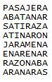
*** 1 8-By-8 square published in 1965 by Dmitri Borgmann [BOR, Language on Vacation, p.198].
PASAJERA : noun : female traveler
ABATANAR : from the verb abatanar (infinitive form) meaning full cloth
SATIRAZA : noun : fat, witty woman
ATINARON : from the verb atinar (third person plural simple past form) meaning hit the mark : (they) hit the mark
JARAMENA : feminine adj. : related to Jarama River in Spain. Example of use : "La ganaderia jarameña de toros"
ENARENAR : from the verb enarenar (infinitive form) meaning cover with sand
RAZONABA : from the verb razonar (third person singular imperfect form) meaning reason : (he) was reasoning
ARANARAS : from the verb arañar (second person singular imperfect subjunctive form) meaning scratch : (that you) would scratch, or (that you) would scratch, or (if you) scratched, or (if you) were to scratch
B3.5. Latin crossword puzzles :
Word squares (two 11-By-11 word squares) :
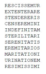
*** Figure 1 : 11-By-11 word square published in 2020 by Eric Tentarelli [TEN].
Warning: this square contains a typo in the display : the second R of the horizontal word STERILITARI must be changed to T [RPR].
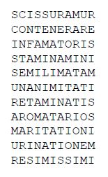
RESCISSEMUR : from the verb rescisso (first person plural future passive form) meaning discover (something unexpected)
EXTENTERARE : from the verb extentero (infinitive form) meaning disembowel
STENDERESIS : from the verb stendo (second person singular imperfect passive subjunctive form) defined as an apheretic form of extendo, a versatile verb whose primary meaning is extend or stretch out.
CENSEREMINI : from the noun censeo (second person plural imperfect passive subjunctive form) meaning value, esteem
INDEFINITAM : from the adjective indefinitus (feminine accusative singular form) meaning indefinite
STERILITATI : from the noun sterilitas (dative singular form) meaning sterility
SERENITATIS : from the noun serenitas (genitive singular form) meaning serenity. This particular inflected form may be familiar because Mare Serenitatis is one of the most visible features on the Moon.
EREMITARIOS : from the adjective eremitarius (masculine accusative plural form) meaning living a hermit's life
MARITATIONI : from the noun maritatio (dative singular form) meaning wedding or marriage
URINATIONEM : from the noun urinatio (accusative singular form) meaning urination
RESIMISSIMI : from the adjective resimus (masculine genitive singular of the superlative form) meaning turned up or bent back, which typically describes noses.
An alternative square is to change EXTENTERARE to EXTENTERATE (second person plural present imperative form of the same verb) and URINATIONEM to UTINATIONEM (accusative singular form of the noun utinatio meaning wish or expression of a wish).
*** Figure 2 : 11-By-11 word square published in 2020 by Eric Tentarelli [TEN].
SCISSURAMUR : from the verb scissuro (first person plural present passive form) meaning cut (cloth, as to make garments)
CONTENERARE : from the verb contenero (infinitive form) meaning make tender
INFAMATORIS : from the noun infamator (genitive singular form) meaning slanderer
STAMINAMINI : from the verb stamino (second person plural present passive form) meaning spin (thread) or support (a vine) with stakes
SEMILIMATAM : from the adjective semilimatus (feminine accusative singular form) meaning half-polished
UNANIMITATI : from the noun unanimitas (dative singular form) meaning unanimity
RETAMINATIS : from the verb retamino (second person plural present form) meaning befoul, particularly with excrement
AROMATARIOS : from the noun aromatarius (accusative plural form) meaning dealer in spices or apothecary
MARITATIONI : from the noun maritatio (dative singular form) meaning wedding or marriage
URINATIONEM : from the noun urinatio (accusative singular form) meaning urination
RESIMISSIMI : from the adjective resimus (masculine genitive singular of the superlative form) meaning turned up or bent back, which typically describes noses.
B3.6. Serbian crossword puzzles :
Word squares (2 10-By-10 word squares) :
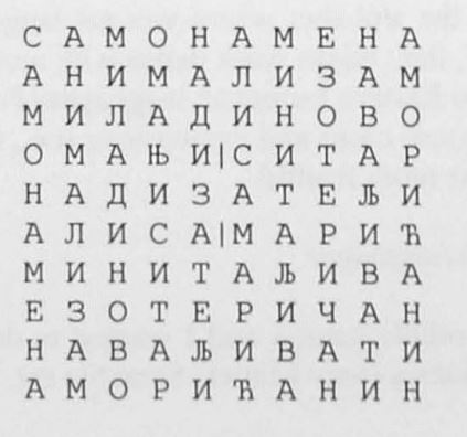
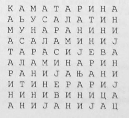
These squares, together with the Croatian squares of Anton Ferderber and Boris Babic, were published in 1999 by Miroslav Lazarevic [NAZ][ECK, The polyglot ten-square].
* 1 10-By-10 word square published in 1987 by Miroslav Lazarevni [NAZ][ECK, The polyglot ten-square][TWO]. Translation by [PER].
SAMONAMENA : noun :
1. sole purpose
2. unique destination
3. exclusive intent
ANIMALIZAM : noun : animalism
MILADINOVO : proper noun :
1. Miladinovo Brdo, hill, 44 04'N, 21 28'E, located near the village of Balajnac, Despotovac Municipality, Pomoravlje district, Serbia.
2. Miladinovo, village, Kardzhali Municipality, Kardzhali Province, Bulgaria, 41 42'N, 25 36'E
OMANJI SITAR : phrase : little sitar
NADIZATELJI : noun : those who surprise from above ?
ALISA MARICH : proper noun : Serbian chess player and Minister of Youth and Sports in the Serbia Government in 2012
MINI TALJIVA : phrase : miniature dissolving object ?
EZOTERICHAN : adj. : esoteric
NAVALJIVATI : verb : to push, to insist
AMORICHANIN : noun : devotee of Cupid ?
* 1 10-By-10 word square published in 1996 by Zivota Stankovic [NAZ][ECK, The polyglot ten-square][TWO]. Translation by [PER].
KAMATARINA : adj. : usurer's
ABUSALATIN : noun : another name for the plant Ricinus communis. This term comes from the Arabic "habb" (grains) and "sultan" (sultan) which refers to the "grains of the sultans" (see https://jezikoslovac.com/ ).
MUNARANINI : noun : little minaret ?
ASALAMINIJ : phrase : and the salamis for me ?
TARASIJEVA : adj. : Tarasije's (Tarasije = Serbian form of the Greek first name Tarasios of Constantinople)
ALAMINARIN : adj. : without laminarin (laminarin = polysaccharide of brown algae)
RANI JANJANI : phrase :
1. ancient Janjani (Janjani = locality, Srebrenik Municipality, Republika Srpska, Bosnia and Herzegovina, 42 13'N, 17 28'E)
2. early Janja inhabitants (Janja = locality, Bijeljina Municipality, Republika Srpska, Bosnia and Herzegovina, 44 40'N, 19 15'E)
3. early Janja supporters (Janja = Janja Bec Neumann, Serbian sociologist and genocide researcher, Nobel Peace Prize winner in 2005)
ITINERARIJ : noun : itinerary
NINIVINICA : phrase : not even a small wine ?
ANIJANIJAC : noun : little spell ? (anijanij = a spell in Marshall islands language)
B3.7. Croatian crossword puzzles :
Word squares (2 11-By-11 and 6 10-By-10 word squares, partial display) :
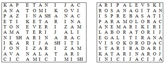
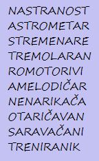
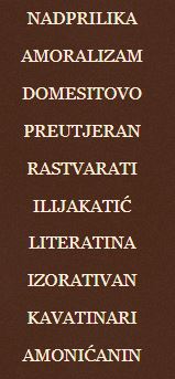
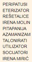
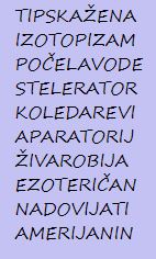

* 1 11-By-11 word square produced in 2015 by Milutin Tepsic [SRP]. Translation conforms to the definitions of this square [SRP].
KAPETANIJAC : noun : the man who lives in the captaincy
ANATOMIKOVI : noun : those who belong to an academician (= anatomist's group ?)
PAZI NA SHANAC : phrase : the soldier, a guard in the trench (ditch) (= watch the trench ?)
ETIKETARINA : noun : the fee that is paid for affixing labels
TONEVERIZAM : noun : Verism heavy as thunder
AMATERIJALI : adj. : immaterials
NISHARINARAC : noun : the toll collector of the Nichava bridge
IKARIJASHITI : verb : to fly too close to the sun
JONIZARIZAM : noun : doctrine advocating widespread ionization
AVANALATARI : noun : mortar tool manufacturers
CICA MICI MISH : phrase : the modern form of the saying "Render unto Cesar what is Cesar's, to God what is God's - literally, "to the cat what it likes most to hunt" (= to the kitty its mouse ?)
* 1 11-By-11 word square produced in 2015 by Zarka Dokica [CVE]. Translation conforms to the definitions of this square [CVE].
ARI PALEVSKI : proper noun : collaborator on the film "Virginity" (2014) directed by Saeed Khoze.
ROSANA GITAN : proper noun : compound female name, the namesake of the Swedish actresses Munter and Goding.
ISPREBASATI : verb : to break out
PARAMOLORAC : noun : resident of Paramo Lora region, Cantabria Province, Spain.
ANEMARI KIRI : proper noun : Austrian humanitarian and author of the book "My Unusual Journeys - Steps of Hope" about her experiences in the 1991-1995 war.
LABORATORIJ : noun : laboratory
EGALITIRANA : verbal adj. : equalized
VISOKORODAC : noun : vegetable plants with tall trees or stems, for example corn.
STARI RADARI: phrase : obsolete radio-locators
KATARINA ROJ : proper noun : a young member of the women's hockey club "Boston Samrocks"
INICIJACIJA : noun : customs and rites (almost among all primitive peoples) by which a boy is declared a boy, and a girl a girl.
* 1 10-By-10 NASTRANOST word square produced in 1941 by Anton Ferderber [DNE][NAZ].
* 1 10-By-10 NADPRILIKA word square produced in 1984 by Boris Babic [BLO][NAZ].
* 1 10-By-10 PERIPATUSI word square produced in 1987 by Boris Babic [ENI][NAZ].
* 1 10-By-10 TIPSKAZENA word square produced in 2010 by Antun Cvitkovic [DNE][DNE2][NAZ].
* 1 10-By-10 OSTANIDOMA word square produced in 2020 by Boris Babic, Resad Besnicanin, Zarko Dokic, Antun Juric, Nedjeljko Nedic, Ilija Ozdanovac and Georgi Zeravica [DOM].
* Other 10x10 word squares including that of Zarka Dokica [CVE].
B3.8. Hungarian crossword puzzles :
Classic crossword puzzles (1 9-By-9 crossword puzzle) :
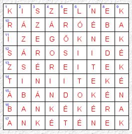
* 1 9-By-9 crossword puzzle published by CPT [CPT]. Translation by [PER].
Horizontally :
KI SZELNEK : phrase : "who are cutting ?"
RAZAROEBA : ?
IZEGOKNEK : ?
SAROSIIDE : adj. : Saros's (Saros = former department of Hungary, 49 00'N, 21 14'E)
ZSEREITEK : adj. : Zs re's (Zs re = another name for Zirany, Nitra region, Slovakia, 48 23'N, 18 10'E)
TINIITEKE : phrase : to your teenagers
ABANDOKEN : ?
BANKEKERA : phrase : towards the bank group ?
ANKETENEK : phrase : for his/her survey
Vertically :
KRISZTABA : phrase : into Kriszta (Kriszta = diminutive of Krisztina)
IAZASIBAN : phrase : while braying
SZERENANK : ?
ZAGORINKE : proper noun : Zagorin's ?
EROSEIDET : phrase : your strong ones ?
LOKI I TOKE : phrase ? : the Loki bow and its arrow rest ?
NENITEKEN : phrase : on your aunt
EBEDEKERE : phrase : towards your lunches ?
KAKEKENAK : ?
B3.9. Hebrew crossword puzzles :
Classic crossword puzzles (1 10-By-10 crossword puzzle) :
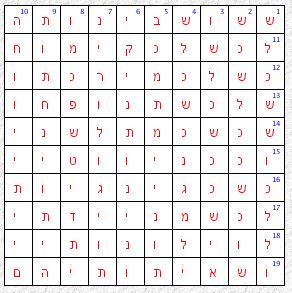
* 1 10-By-10 crossword puzzle published by CPT [CPT]. Partial list of words translated by [PER] :
Horizontally :
1- she shoshbinotayikh : phrase : "who are her bridesmaids ?"
12- keshelkhem yirkhtu : phrase : when it belongs to you, they buy it
19- ve se ototeihem : phrase : and that theirs signs
Vertically :
1- shel keshe shukhlelu : phrase : of when they were perfected
10- ha havayati'im : phrase : the experiential aspects
B3.10. German crossword puzzles :
Word squares (4 7-By-7 word squares) :
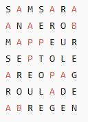
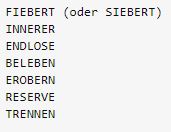
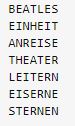
*** 1 7-By-7 crossword puzzle published in 2022 by the magazine Süddeutsche Zeitung [SUD].
SAMSARA : noun : samsara
ANAEROB : adj. : anaerobic
MAPPEUR : noun : mapper
SEPTOLE : noun : septuplet (musical technical term)
AEROPAG : noun : Areopagus (supreme court in ancient Athens)
ROULADE : noun : roulade
ABREGEN : verb : to cool down
*** 2 7-By-7 crossword puzzles (with alternative) created by Tim in 2022 [GIB].
FIEBERT : conjugated verb : (he) has a fever. An alternative square uses SIEBERT meaning (regional technical term) : (he) filters.
INNERER : declined adj. : inner
ENDLOSE : declined adj. : endless
BELEBEN : verb : to revive
EROBERN : verb : to conquer
RESERVE : noun : reserve
TRENNEN : verb : to separate
* 1 7-By-7 crossword puzzle created by Tim in 2022 [GIB].
BEATLES : proper noun : Beatles
EINHEIT : noun : unit
ANREISE : noun : journey
THEATER : noun : theater
LEITERN : noun : ladders
EISERNE : adj. : iron
STERNEN : declined noun : stars
Sources relating to crossword puzzles :

B4.1. Introduction :
Mnemonics encompasses all the techniques designed to facilitate the memorization and recall of information through mental associations.
Among these methods, the number articulation method [WIK] stands out for its effectiveness in remembering numbers. This system is based on a fixed correspondence between the numbers 0 to 9 and consonant sounds. For example, 3 corresponds to the sound "m". By freely adding vowels, sequences of numbers are transformed into concrete words that are easier to memorize. For example, the number 42 can become the word mouton (m = 3, t = 1).
The recall table of figures (from 0 to 9) was developed in the 19th century by Aimé Paris [PAR, p.28] and then adopted identically by Abbé François-Napoléon-Marie Moigno [WIK]. A different, simpler version was later proposed by Joe Bertin [BER] in 2028, and adopted almost identically by Régis Petit in 2025.
The recall table of numbers from 00 to 99 assigns a specific word to each of these numbers.
The steps of the number articulation method are as follows :
1. Associate each number from 0 to 9 with a consonant sound, according to a code to be memorized (see Recall table of figures).
2. Convert the sequence of numbers to be memorized into a sequence of sounds, according to this code.
3. Form a sequence of words from these sounds by adding vowels, so as to phonetically create a sentence, or mentally create a vivid and memorable story.
4. To reproduce the numbers, proceed in reverse : story, words, sounds, numbers.
Example of a story in French that you can create yourself to remember the first decimals of the number Pi = 3, 14 15 92 65 35 89 79 32 38... :
- According to the recall table of figures by Aimé Paris : "assis par TeRre sur une modeste ToiLe, je suis en PaNne et GèLe. Au loin, près d'une MeuLe de foin, se trouve une VamP portant une CaPe de MoiNe et des MouFles."
- According to the recall table of figures by Régis Petit : "sur mon TanK, à côté d'une TaSse, d'une PoiRe et d'une GouSse d'ail, j'écoute la MeSse, quand surgit un BiP sonore. J'éclaire avec ma LamPe et vois une MaRe avec un MeuBle en plein milieu."
Applications :
Among the applications where the number articulation method provides real benefits, we can cite :
- Telephone numbers encoded into 5 concrete words of two digits each (example : 06 12 34 56 78)
- Anniversary dates encoded into 4 concrete words (example : 24 02 1958)
- Access codes (PIN code, building door code, safe code, alarm code, etc.) encoded into 2 or 3 concrete words depending on their length
- Social security numbers encoded into an initial digit (gender : 1 male, 2 female) followed by 7 concrete words (example : 1 58 02 XX XX XX XX XX)
B4.2. Recall tables of figures from 0 to 9 :
The recall table of figures from 0 to 9 is not unique and depends on its author :
- Aimé Paris's table has the merit of codifying all common consonant sounds. The association between figure and sound(s) must be memorized.
- Joe Bertin's table associates a consonant letter with each figure, which provides a visual aid that greatly facilitates sound memorization.
- Régis Petit's table reproduces Joe Bertin's table, modifying the letters associated with the figures 2 and 4, which improves the visual aid (see Figure above).
The different tables are as follows :
Table legend : (*) according to the orthographic writing of the phonemes.
| Figure | Song (*) and image according to Aimé Paris [PAR, p.28][WIK][APP] | Other image according to Régis Petit | Song (*) and image according to Joe Bertin [BER] | Song (*) and image according to Régis Petit |
|---|---|---|---|---|
| 0 | "s" or "z", one of the loops of the letter s | SanS aide | "d", letter D | "d", letter D |
| 1 | "t" or "d", single leg of the letter t | TenDu ou Tout Droit | "t", letter T | "t", letter T |
| 2 | "n" ou "gn", double leg of the letter n | Na ! (attitude enfantine de provocation) | "n", letter N sideways | "r", letter R without a vertical bar |
| 3 | "m", triple leg of the letter n | Maman | "m", letter M sideways | "m", letter M sideways |
| 4 | "r", upside-down or mirrored letter r | trois Ratures faites avec Rage | "r", letter R mirrored | "k", letter K (with a block of three strokes) |
| 5 | "l", similar to the letter L in French cursive round writing [LIV1][LIV2] | Ligne verticale ratatinée | "s", letter S | "s", letter S |
| 6 | "ch" or "j", similar to the letter j in French cursive round writing [LIV1][LIV2] | Chat qui Jaillit | "g" ou "j", letter G | "g" ou "j", letter G |
| 7 | "k" or "g", gallows shape similar to the letter q or g | Coups Guerriers (indiqués par deux Coupures) | "l", letter L upside-down | "l", letter L upside-down |
| 8 | "f" or "v", similar to the letter F in French cursive round writing [LIV1][LIV2] | FèVe (sous forme de petit enFant) | "b", letter B | "b", letter B |
| 9 | "p" or "b", mirrored letter p or upside-down letter b | Petit Bébé (en position foetale avec sa grosse tête) | "p", letter P mirrored | "p", letter P mirrored |
B4.3. Recall tables of numbers from 00 to 99 :
Anyone can freely construct their own recall table of numbers from 00 to 99, based on a given recall table of figures.
The recall tables of numbers from 00 to 99 proposed below were created by Régis Petit. The first is based on Aimé Paris's coding of figures, the second on Régis Petit's coding of figures.
These two tables are designed according to the following rules for easy memorization of concrete words :
Concrete word = common or proper noun, with a single syllable of the CVC or CSVC type, such as :
C = consonant associated with the figure in the recall table of figures.
V = vowel that can be (*) : "é" "è" "eu" "in" "a" "an" "ou" "o" "on" "i" "u"
S = semi-consonant at the onset of a V vowel, which can be (*) : "w" "y" "u+"
The V or SV nucleus of the syllable is chosen primarily from the sounds (*) : "é" "è", "eu", "in"; "a", "an" ; "ou", "w" V ; "o", "on" ; "i", "y" V ; "u", "u+" V
(*) according to the orthographic writing of the phonemes.
Exceptions to these rules are in italics in these tables.
| Number | Concrete word conforming to Aimé Paris's coding of figures | Concrete word conforming to Régis Petit's coding of figures |
|---|---|---|
| 00 | Sas | Dinde |
| 01 | Soute | Datte |
| 02 | Scène | Dard ou Dur |
| 03 | Somme | Dame |
| 04 | Serre ou Soeur | Dock ou Duc |
| 05 | Selle | Danse |
| 06 | Souche | Danger ou Dingue |
| 07 | Sac | Dalle |
| 08 | Soif | Dab ou Daube |
| 09 | Sep | Dieppe ou Dupe |
| 10 | Tasse | Tiède |
| 11 | Tête ou Tente | Tête ou Tente |
| 12 | Tonne | Terre |
| 13 | Tome | Tome |
| 14 | Terre | Tank |
| 15 | Toile | Tasse |
| 16 | Tache | Tige ou Tag |
| 17 | Tank | Toile |
| 18 | Touffe | Tombe |
| 19 | Taupe | Taupe |
| 20 | Nasse | Rade |
| 21 | Natte | Rate |
| 22 | Nonne | Rire |
| 23 | Nem | Rame |
| 24 | Nerf | Rack |
| 25 | Nul | Race |
| 26 | Niche | Rage ou Reg |
| 27 | Nuque | Râle |
| 28 | Nef | Rab ou Robot |
| 29 | Nappe | Rampe ou Repas |
| 30 | Messe | Mode |
| 31 | Meute ou Motte | Meute ou Motte |
| 32 | Moine | Mer ou Mare |
| 33 | Môme | Môme |
| 34 | Mer ou Mare | Mec |
| 35 | Meule ou Malle | Messe |
| 36 | Mèche | Mage ou Mangue |
| 37 | Mec | Meule ou Malle |
| 38 | Moufle | Meuble |
| 39 | Myope | Myope |
| 40 | Race | Coude |
| 41 | Rate | Quinte ou Côte |
| 42 | Reine | Coeur |
| 43 | Rame | Came |
| 44 | Rire | Cake |
| 45 | Râle | Caisse |
| 46 | Roche | Cage |
| 47 | Rack | Cale |
| 48 | Rouf ou Rêve | Cube |
| 49 | Râpe | Coupe ou Cape |
| 50 | Laisse | Soude |
| 51 | Latte | Soute |
| 52 | Laine | Serre ou Soeur |
| 53 | Lame | Somme |
| 54 | Lard | Sac |
| 55 | Lille | Sas |
| 56 | Louche | Singe ou Sangle |
| 57 | Lac | Sel |
| 58 | Lymphe | Sabre |
| 59 | Loupe | Soupe |
| 60 | Chasse | Jade ou Guide |
| 61 | Jante ou Chatte | Jatte ou Goutte |
| 62 | Jeune ou Chaîne | Jour ou Gare |
| 63 | Gym ou Chaume | Gym ou Gamme |
| 64 | Jour ou Chair | Jonque |
| 65 | Gel ou Châle | Gousse |
| 66 | Juge | Juge ou Gong |
| 67 | Jonque ou Chèque | Gel ou Gueule |
| 68 | Chef | Jambe |
| 69 | Jupe ou Chappe | Jupe ou Guêpe |
| 70 | Caisse | Lad ou Lande |
| 71 | Quinte ou Côte | Latte |
| 72 | Canne | Lard |
| 73 | Came | Lame |
| 74 | Coeur | Lac |
| 75 | Cale | Laisse |
| 76 | Couche | Linge ou Langue |
| 77 | Cake | Lille |
| 78 | Coiffe | Lobe |
| 79 | Coupe ou Cape | Lampe |
| 80 | Fesse | Bande |
| 81 | Fête | Bête |
| 82 | Fouine | Beurre |
| 83 | Femme | Boum |
| 84 | Fer | Banque |
| 85 | Foule ou Fil | Bosse |
| 86 | Fiche ou Vache | Bouge ou Bague |
| 87 | Fac | Balle |
| 88 | Fief | Bob |
| 89 | Vamp | Bip |
| 90 | Pince | Panda ou Poudre |
| 91 | Patte | Patte |
| 92 | Panne | Poire |
| 93 | Pomme | Pomme |
| 94 | Père | Pack ou Pique |
| 95 | Pelle | Panse |
| 96 | Pêche | Page |
| 97 | Pack ou Pique | Pelle |
| 98 | Pouf | Pub ou Poubelle |
| 99 | Pape ou Poubelle | Pape |
B4.4. Sources relating to Mnemonics :
[APP] Apprendre5minutes, Comment mémoriser facilement les chiffres ou les nombres
[BER] Joe Bertin, Astuce de mémorisation : la table de rappel
[LIV1] French Handwriting Schoolbook, écriture ronde française
[LIV2] pilllpat (agence eureka), album Alphabete
[PAR] Aimé Paris, Exposition et pratique des procédés mnémotechniques à l'usage des personnes qui veulent étudier la mnémotechnie en général comme un moyen d'abréger l'étude de toutes les connaissances humaines, Paris, 1825
[WIK] Wikipedia, Code chiffres-sons
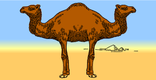
B5.1. Introduction :
A palindrome is a form of linguistic symmetry where a sentence (which can be as short as a single word) reads or sounds the same in both directions. See Attributed palindromic sentences, Anonymous palindromic sentences, Palindrome cities and Palindrome first names.
Orthographic palindromes are based on the order of letters in writing, as in "C'est sec".
The same applies to word palindromes that are based on the order of words in writing, as in "Un pour tous, tous pour un" or in "La juste est juste là" (for a non-strict palindrome).
The same applies to syllabic palindromes at the syllable pronunciation level, as in "Laconique Nicolas", corresponding to the syllabic sequence "la" "ko" "ni" "ke" "ni" "ko" "la".
The same applies to phonetic palindromes at the phoneme pronunciation level, as in "Il aima Amélie", corresponding to the phonetic sequence "i" "l" "é" "m" "a" "a" "m" "é" "l" "i".
The same applies to numeric palindromes at the writing level, as in the date "02/02/2020".
The same applies to Rotational palindromes at the writing level, as the word "inoui".
The same applies to mirror palindromes which read identically after reflection in a mirror.
The same applies to musical palindromes at the level of the notes of the musical phrase.
The palindromes listed below are exclusively orthographic palindromes in the French language, where case (upper/lower case), diacritical marks (accent, diaeresis, cedilla, tilde, etc.), spaces and punctuation marks (period, comma, dash, parentheses, etc.) are not taken into account.
B5.2. Attributed palindromic sentences :
The most beautiful palindromic sentences in the French language, attributed to an author, are the following :
A Cuba, Anna a bu ça (Gérard Durand).
A Laval, elle l'avala (Michel Laclos).
A l'étape, épate-la ! (Louise de Vilmorin).
A révéler mon nom, mon nom relèvera (Edmond Rostand, dans Cyrano de Bergerac).
Ce satrape repart à sec (Pierre Bailly).
C'est sec (Roger Cornaille).
Eh ! ça va la vache ? (Louise de Vilmorin).
Elisa, là, à l'asile (Lennig Gullon).
Elu par cette crapule (Charles Cros).
Emile-Eric, notre valet, alla te laver ton ciré élimé (Georges Perec).
Engage le jeu que je le gagne (Alain Damasio).
En nos repères, n'insère personne (Dominic Bergeron).
En route je tourne (Roger Cornaille).
Eric, notre valet, alla te laver ton ciré (Jacques Capelovici).
Esope reste ici et se repose (Jacques Capelovici).
Etel, un port trop nu, l'été (Claude Gaignière).
Et la Marine va venir à Malte (attribué à Victor Hugo).
Et Luc colporte trop l'occulte (Michel Laclos).
Karine égarée rage en Irak (Gérard Durand).
Karine libre à Erbil en Irak (Christophe L.)
La Marine en ira mal (attribué à Victor Hugo).
La mariée ira mal (Louise de Vilmorin).
L'âme des uns n'use de mal (Etienne Pasquier).
L'amer vin enivre mal (Jean T.).
La mère Gide digère mal (Louis Scutenaire).
L'âme sûre ruse mal (Louise de Vilmorin).
L'ami naturel ? Le rut animal ! (Louise de Vilmorin).
Lune de ma dame d'été, été de ma dame de nul (Louise de Vilmorin).
Nier est effet serein (Stéphane Susana).
Noël a trop par rapport à Léon (Sylvain Viart).
Oh ! cet écho (André Tomkins).
Par-delà le drap (Patrick Hospital).
Rions noir (Jacques Bens).
Rue Verlaine gela le génial rêveur (Jacques Perry-Salkow).
Ta bête te bat (Louise de Vilmorin).
Un art luxueux ultra nu ! (Matthieu Godbout).
Un émir fada, venu du Nevada, frime nu (Gérard Durand).
B5.3. Anonymous palindromic sentences :
The most beautiful palindromic sentences in the French language, without a known author, are the following :
A l'autel elle alla, elle le tua là.
Bon sport, trop snob.
Car, tel Ali, il a le trac.
Ce mec.
essayasse.
Etna : lave dévalante.
Etre là, alerte.
Et se resservir, ivresse reste.
Et Tesio, né borné et naïf, emporte une vedette devenue trop méfiante en robe noisette (Francis Pacherie).
Ici.
Il a pâli.
Il a sali.
Karine alla en Irak.
L'âge légal.
La malade pédala mal.
L'âme d'Eve rêve de mal.
La mère puce récupère mal.
L'âne vénal.
malayalam (langue parlée en Inde).
mon nom.
Nie, reste net, serein.
Ni lac, ni patelin, ni le tapin câlin.
Oh ! Cela te perd, répéta l'écho.
ressasser.
Réussir à Paris : suer.
rotavator.
S'engager à revers : rêver à regagnes !
Sexe vêtu, tu te vexes ?
Ta belle porte s'use trop, elle bat.
Trace là mon nom à l'écart.
Un drôle de lord nu.
Un ému a son os au menu.
Un enfer bref. Né nu.
Un été nu.
Un rêve de ver nu.
Un roc lamina l'animal cornu.
Un roc si biscornu.
Zeus a été à Suez.
B5.4. Palindrome cities :
The main palindrome cities of the world are the following :
Allemagne : Burggrub (Bavière), Hammah (Basse-Saxe), Mussum (Rhénanie-du-Nord-Westphalie), Woddow (Brandenburg), Zeez (Mecklenburg-Vorpommern)
Angola : Seles (Cuanza Sul)
Arabie Séoudite : Al'Ula (Madinah)
Argentine : Neuquén (Patagonie)
Australie : Aramara (Queensland), Arrawarra (Nouvelle-Galles-du-Sud), Civic (Territoire de la Capitale Australienne), Glenelg (Adélaïde, Australie-Méridionale), Hattah (Victoria), Lal Lal (Victoria), Parap (Territoire du Nord), Paraparap (Victoria), Tumut (Nouvelle-Galles-du-Sud)
Belgique : Eke, Ellemelle (Province de Liège), Ere
Brésil : Aba (Bahia), Acaiaca (Minas Gerais), Aia (Ceara), Mutum (Minas Gerais)
Burkina Faso : Bob (Région du Centre-Ouest)
Canada : Elôle (Québec), Kinikinik (Alberta), Laval (Québec), Navan (Ontario), Salas (Nouvelle-Ecosse), Wakaw (Saskatchewan)
Chili : Lolol (O'Higgins)
Chine : Nan'an (Fujian)
Danemark : Dragsgard, Vellev
Egypte : Aga (gouvernement de Daqahliyya)
Espagne : Aba (Pays basque), Aja, Aya, Oco, Ollo (Navarre), Oro, Oso (Catalogne), Salas (Asturie), Saras, Senés (Andalousie), Sotos
Etats-Unis : Ada (Oklahoma, Oho, Minnesota), Ala (Alabama), Anna (Ohio, Texas, Illinois), Ava (Missouri, Illinois, New York), Capac (Michigan), Civic (Canberra), Eleele (Hawaï), Hannah (Michigan, Dakota du Sud, Caroline du Nord), Harrak (Oklahoma, Washington), Ixixi (Alaska), Kanakanak (Alaska), Kinikinik (Colorado), Level (Ohio, Maryland), Noxon (Montana), Otto (plusieurs Etats), Oto (Iowa), Remer (Minnesota), Renner (Texas), Wassamassaw (nom d'une région de Caroline du Sud)
Ethiopie : Asasa, Asosa
Finlande : Asa (Laponie), Esse, Ii (Ostrobotnie), Orö
France : Afa, Callac, Esse, Eve, Eze, Laval, Noron, Noyon, Oô, Sajas, Sanas, Saras, Savas, Sées, Selles, Senones, Serres, Sos, Sus
Grèce : Sedes, Serres
Groenland : Qaanaaq (Région Qaasuitsup)
Hongrie : Tat, Tét, Pap, Ziliz
Inde : Ara (Bihar), Aramara, Atta (Uttar Pradesh), Aya (Maharashtra), Gadag (Karnataka), Idappadi (Tamil Nadu), Itamati (Odisha), Rapar (Gujarat), Nawagawan
Iran : Barab, Basab, Kahak, Karak, Kuruk, Naran, Qoroq, Sarras, Selles, Sis, Sus, Tabbat
Irlande : Navan (Comté de Meath)
Israël : Akka, Na'an
Italie : Ala (Trentin-Haut-Adige), Ateleta (Abruzzo), Erre (Podesteria, ancien nom), Onano (Latium), Onno (Lombardie), Sennes (Tyrol du Sud), Siris (Calabre)
Japon : Aka (Fukuoka), Akasaka (Tokyo, Okayama), Ama (Shimane), Awa (Tokushima), Ono (Préfecture de Hyogo)
Mali : Tamahamat, Tassassat
Maroc : Akka, Assa
Mauritanie : Tétêt (Région de l'Adrar)
Niger : Tabadabat, Tassessat
Nigeria : Aba (Etat d'Abia), Abiriba, Apapa, Elele (Rivers), Irri, Ososo, Oyo (Etat d'Oyo)
Nouvelle-Zélande : Aka Aka (Auckland)
Pays-Bas : Ede (Province de Gueldre), Ee (Province de Groningue), Epe (Province de Gueldre)
Pologne : Wolow (Basse-Silésie)
République tchèque : Vokov
Roumanie : Anina (Judet de Caras-Severin)
Royaume-Uni : Anna (Suffolk), Eve (Ecosse), Eye (Cambridgeshire, Suffolk), Glenelg (Ecosse), Notton (West Yorkshire, Angleterre)
Russie : Aga (République de Sakha) Tommot (Iakoutie), Ulu (Iakoutie), Yessey (Krasnoïarsk)
Sénégal : Matam (Région de Matam)
Suède : Abba (Province de Dalécarlie), Dörröd, Kivik, Murum
Suisse : Planalp (Obwald)
Thaïlande : Nan (Province de Nan)
B5.5. Palindrome first names :
The main palindrome first names are the following :
Legend : (*) indicates the most common palindrome first names in France (born in France or listed in the INSEE "First Names" database since 1900).
Female first names :
Ada (*), Adda
Aa
Anevena
Anina
Anona
Arezera
Afifa
Aviva
Aia, Aya
Arora
Atta
Ece
Elle (*)
Eve (*)
Hawah, Hawwah
Immi
Ireri
Ivi
Izzi
Layal
Lenel
Malayalam
Maram
Okko
Viv
Male first names :
Aba, Abba
Alla
Aoloa
Bob (*)
Did
Efe
Lehel
Nan
Natan (*), Nattan
Nayan
Neven
Odo
Oto, Otto (*)
Reber
Reinier
Sabas
Savas
Talat, Tanat
Unisex first names :
Aja (*)
Ama (*), Amma
Ana (*), Anna (*), Anena, Hannah (*)
Ara
Asa
Ava (*), Awa
Axa
Aza, Azza, Aziza
Civic
Ebbe
Ede
Eme, Emme (*)
Görög
Kajak, Kayak
Lil (*), Lyl
Noon
Nosson
Ono
Siris
Uru
Yay
Zaz
B5.6. Word palindromes :
Word palindromes are phrases that read identically from right to left and from left to right at the word level, regardless of case (upper/lower case) and punctuation marks (period, comma, dash, parentheses, etc.), as in the following examples :
Un pour tous, tous pour un
Papa aime maman, maman aime papa
Nous avions les avions, nous !
Pierre baise à Baise-Pierre
Some word palindromes, less strict, allow the omission of diacritical marks (accent, diaeresis, cedilla, tilde, etc.), as in the following examples :
La juste est juste là
La foule, foule-là !
Saint-Pierre a marié Marie à Pierre Saint
B5.7. Numeric palindromes :
The major numeric palindrome are the following [PAL][VIL] :
02-02-2020
21-12-2112
121 = 38 + 83 = 121
12 345 678 987 654 321 which is the square of palindromic number 111 111 111
982 623 644 294 744 275 088 611 239 676 071 787 170 676 932 116 880 572 447 492 446 326 289 which is the square of non-palindromic number 31 346 828 297 209 660 045 268 842 120 992 233 (July 5, 2024 - Patrick De Geest)
1 030 607 060 301 which is the cube of palindromic number 10 101
1 331 000 039 930 000 399 300 001 331 which is the cube of palindromic number 1 100 000 011
10 662 526 601 which is the cube of non-palindromic number 2 201
B5.8. Rotational palindromes :
Rotational palindromes (also called "rotational ambigrams") are words or phrases that read identically after rotating the entire set halfway.
This property applies exclusively to the following characters [AMB][DEL] :
Digits : 0, 1, 8, which remain invariant under rotation, and 6/9 which are rotation pairs of each other.
Punctuation marks : - : () [] {} which remain invariant under rotation.
Symbols : + - / x = ≠ ∞ \ ∫ ⊗ # $ % | θ ι ο χ which remain invariant under rotation.
Capital letters : H, I, N, O, S, X, Z, which remain invariant under rotation, and M/W which are rotation pairs of each other.
Lowercase letters : i, l, o, s, x, z, which remain invariant under rotation, and a/e, b/q, d/p, h/y, m/w, n/u, which are rotation pairs of each other.
The most beautiful rotational palindromes are the following :
NON
SOS
SONOS
NOW NO SWIMS ON MON (qui signifie "Maintenant plus de piscine le lundi")
NeW MaN
aie
axe
aune
yeah
apode
inoui
sales
saxes
suons
nounou
salles
saisies
saillies
elle alla
andin basnoda a une épouse qui pue (Georges Perec).
Note that some words can give rise to another word by rotating it halfway. Examples :
91 = 90 + 01 / 10 + 06 = 19
NOM/WON
NOS/SON
las/sel
epis/sida
eues/sana
iles/sali
oued/pano
sans/sues
ailes/salie
aillé/allié
esses/sassa
assassins/suissesse
le pou / nodal
Also note that some words can give rise to the same word or another word by rotating them a quarter turn. Examples :
Counterclockwise (where the capital letters C E H I M N O X Z become respectively U W I H E Z O X N) :
OHIO/OHIO
MON/ZOE
ZOE/WON
con/cou
Clockwise (where the capital letters E H I N O U W X Z become respectively M I H Z O C E X N) :
OIE/OHM
ZOE/NOM
B5.9. Mirror palindromes :
Mirror palindromes are words or phrases that exhibit axial symmetry, either horizontally or vertically, and read identically when viewed in a mirror held horizontally or vertically.
Horizontal symmetry reverses top and bottom, while preserving left and right and the order of the letters. BEC in a horizontal mirror remains BEC.
Vertical symmetry reverses left and right as well as the order of the letters within the word, while preserving top and bottom. TOUT in a vertical mirror becomes TUOT.
These symmetry properties applie exclusively to the following characters [AMB][DEL] :
Horizontal symmetry :
Numbers : 0, 1, 3, 8
Punctuation marks : . - : () [] {}
Symbols : + - x = > < ∑ ∞ ∫ ⊗ | € ε θ ι κ ο χ
Uppercase letters : B, C, D, E, H, I, K, O, X
Lowercase letters : c, i, k, l, o, x
Vertical symmetry :
Numbers : 0, 1, 8
Punctuation marks : . - : " '
Symboles : + - ± x = * ∏ ∞ ⊗ _ | γ θ ι ν ο π τ υ χ ψ ω
Uppercase letters : A, H, I, M, O, T, U, V, W, X, Y
Lowercase letters : i, l, m, o, u, v, w, x
Examples of mirror palindromes with horizontal symmetry :
BEC
BICHE
DIODE
EXCEDEE
kilo
Examples of mirror palindromes with vertical symmetry :
TOT
AVIVA (3ème personne du singulier du passé simple du subjonctif du verbe aviver
MAOAM (marque de bonbons pâte à mâcher d'origine allemande)
MATAM (ville du Sénégal)
TAMAT (3ème personne du singulier de l'imparfait du subjonctif du verbe tamer)
TATAT (3ème personne du singulier de l'imparfait du subjonctif du verbe tâter)
TAXAT (3ème personne du singulier de l'imparfait du subjonctif du verbe taxer)
HAITI, AH !
MOT A TOM
wow (interjection d'origine anglaise exprimant la surprise ou l'émerveillement)
B5.10. Musical palindromes :
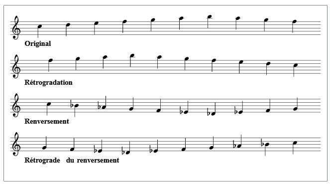
Musical palindromes are sound sequences constructed to remain identical when played in either direction, according to two possible types of symmetry :
- Retrograde (B), which consists of replaying the sequence of notes (A) in reverse order in time. Example (see Figure above) : The original sequence Do Ré Mi Fa Sol La Si La Sol Fa generates the inverse sequence Fa Sol La Si La Sol Fa Mi Ré Do.
- Inversion (C), which consists of replaying the sequence of notes by reversing the direction of the intervals between these notes around an imaginary horizontal axis. Example (see Figure above, with Do chosen as the reference point for the horizontal axis) : The sequence Do Ré Mi Fa Sol La Si La Sol Fa generates the inverse sequence Do Sib Lab Sol Fa Mib Réb Mib Fa Sol.
- The retrograde of inversion (D), which consists of combining these two processes. Example (see Figure above) : The combination of the two previous examples generates the sequence Sol Fa Mib Réb Mib Fa Sol Lab Sib Do.
Warning : Palindromic inversion (C) is different from inversion of an interval or chord in music.
Depending on the composer, pieces A, B, C and D can be mixed in sequence or superimposed. For example :
In Guillaume de Michaut ("My End Is My Beginning") : Superimpose A + B + C', where the Tenor voice is an integral part of A.
In J.S. Bach (Musical Offering, Canon Cancrizans, or Canon Per Motum Contrarium) : Superimpose A + B or sometimes superimpose A + D
In Haydn (Symphony No. 47, Minuet of the Palindrome) : Sequence A then B then C then superimpose A + D
B5.11. Sources relating to Palindromes :
[AMB] Wikipedia - Ambigramme
[DEL] Jean-Paul Delahaye, Ambigrammes, revue Pour la Science, N 323, Septembre 2004
[DUR] Gérard Durand, Palindromes en folie
[PAL] The Palindrome, Palindrome ?
[QUI] Quillbot, Palindromes
[RED] reddit, Quelle est la plus grande ville du monde qui porte un nom palindromique ?
[STA] StarinuX, Liste de palindromes
[VIL] Gérard Villemain, Langue - Palindromes - Villes
[VIL] Gérard Villemain, Formes- Palindromes - Introduction
[VIL] Gérard Villemain, Formes - Palindromes - Dates
[VIL] Gérard Villemain, Formes- Palindromes - Carrés
[VIL] Gérard Villemain, Formes- Palindromes - Cubes
[WIK] Wikipedia, Palindrome
[WIK] Wikipedia, Liste des palindromes en français
[WIK] Wikipedia, Palindrome (multilangues)
Here is a collection of spectacular magic tricks.
Contents :
B6.1. Magic tricks with ropes or rubber bands :
Here are some spectacular tricks using ropes, rubber bands or just your hands.
B6.1.1. Hands turned over :

This trick is a popular cognitive psychology experiment.
A spectator is asked to interlace their fingers, palm to palm, in an inverted position, and then turn them over.
This slightly uncomfortable position exposes both rows of fingers to the upwards (see Figure above).
A specific finger is then pointed out without being touched, and the spectator is asked to raise it quickly and without thinking.
The spectator then frequently raises the opposite, symmetrical finger.
This error arises from a conflict between an internal representation of the fingers, disrupted by the unusual posture, and the automatic motor commands, designed for hands in a normal position. Vision could correct this, but not quickly enough when an immediate response is required.
B6.1.2. Battery swap between two hands :
This dexterity trick involves swapping two round AA batteries from one hand to the other without dropping them or using any special effects.
The manipulation is simple and quick, but difficult for a spectator to reproduce.
The steps are as follows (see Figure above, cf. [PRA][ASH]) :
1. Hold a round AA battery in the crook of each thumb and index finger, pinching the battery in the middle, slightly angled towards the wrist, with the bottom (negative pole) facing the palm.
2. Position your hands facing the spectator, palms hidden, in head-to-tail position, with your fingers horizontal and in a vertical plane.
3. Rotate your right hand a quarter turn counterclockwise.
4. Bring your hands together, keeping your fingers parallel, with your right thumb sliding under your left thumb.
5. Place each thumb on the bottom of each battery and loop each miidle finger over the other end of the batteries (positive pole).
6. Pinch each battery between your thumb and middle finger, then gently separate your hands.
7. Rotate both hands slightly to present the two batteries vertically to the spectator.
8. Return the batteries to their initial position (step 1) by reversing the steps.
Note : Instead of pinching the batteries between thumb and middle finger, you can also do it between thumb and index finger (as shown in the Figure above), but this finger position during the cross-locking (step 5) is more forced and less comfortable.
B6.1.3. The traveling ring :

1. This spectacular trick requires a ring and a cut not-too-bright rubber band approximately 10 cm long (see Figure above, cf. [MIR]).
2. Coil the rubber band in your left hand, leaving about 1 cm of the end sticking out. Pinch the end firmly between your thumb and index finger, then pass the rubber band through the ring.
3. Grasp the rubber band between the thumb and index finger of your right hand, tender it to the maximum, and tilt it slightly upwards. The ring will naturally stop against your left hand.
4. Without moving either hand, the ring will then begin to slowly slide up the rubber band.
Solution : After stretching the rubber band, let it slide gently between the thumb and index finger of your left hand, causing the ring to slide up.
B6.1.4. Bouncy rubber band between fingers :
This magic trick requires a small, brightly colored rubber band.
The steps are as follows (see Figure above, cf. [CAR2]) :
1. Facing the spectator, hold the rubber band above a vertical hand.
2. Loop the rubber band around the index and middle fingers of this hand.
3. Press your fingers and thumb against the rubber band and close your fist, saying this aloud.
4. Blow on your fingers and reopen your fist. The rubber band will suddenly jump and wrap around the other two fingers.
Explanation : Just before closing your fist, grasp the rubber band between the thumb and index finger of your other hand (5a), pull it quickly down to the base of your palm (5b), close your fist (5c), and place the rubber band at the base of your four fingernails, starting with your little finger and working towards your index finger (5d). Then open your fist (5e).
Improved solution : To better conceal this secret manipulation, before closing the fist, grasp the rubber band, pull it back with your index finger while pressing your palm against your wrist, thumb and other fingers facing the spectator, close your fist, lower your arms under the table, place the rubber band on your fingers, re-press the wrist, and show the whole thing unchanged to the spectator. Then open your fist.
B6.1.5. Bouncy rubber band between hands :
This magic trick requires two rubber bands of the same color and quite long.
The steps are as follows (see Figure above, cf. [MAGE]) :
1. Present your open palm to the spectator, with a rubber band around the top of your thumb and the base of your other four fingers.
2. Using the index finger of your other hand, gently peel the rubber band away from your palm to clearly demonstrate that it is normal.
3. Present your other hand upside down and tap your fingers together.
4. Raise your thumb. The rubber band will suddenly jump onto the four fingers of your other hand.
Solution : Prepare the rubber band as follows :
5a. Place the rubber band around your wrist, on the palm side, then in the hollow between your thumb and your index finger.
5b. Press your thumb firmly against your index finger to secure the rubber band, then turn your hand over so your palm is facing up.
5c. Pass the rubber band between the top of your thumb and index finger, maintaining pressure.
5d. Turn your hand over so your palm is facing down, then pass the loop of the rubber band around your four fingers.
5e. Turn your hand over again, palm up, with the rubber band positioned at the base of your four fingers.
5f. Pull the rubber band slightly to pass it over the top of your thumb.
5g. Place a second rubber band around your wrist to conceal the secret preparation.
The preparation is now complete, and the trick can begin in front of a spectator.
B6.1.6. Intertwined rubber bands :
This magic trick requires two small, identical rubber bands of the same color.
The steps are as follows (see Figure above, cf. [JER]) :
1. Hold one rubber band vertically between the thumb and forefinger of your left hand, and another between the thumb and middle finger of your right hand, with the two rubber bands intertwined.
2. Move both hands by bringing them together and moving them apart, and also by rotating them in opposite directions, to show the spectator that the system is locked.
3. Suddenly separate your hands. Both rubber bands will be released.
Solution :
4a. As you rotate your hands, pass your right index finger, which is free, through the loop of your right thumb.
4b. Push your right index finger in and pass it behind the left rubber band.
4c. Remove your right middle finger from the right rubber band.
4d. The rubber band will automatically move over your right index finger.
4e. Immediately press the rubber band against the other one to simulate the lock.
4f. Suddenly move your hands apart.
Improved solution (cf. [PAU][VAL]) :
In step 1, hold the rubber band horizontally (and not vertically), which avoids passing behind the left rubber band in step 4b.
B6.1.7. String handcuffs puzzle :

This spectacular trick is the following :
1. Two people are standing facing each other (see Figure above, cf. [EIT]).
Each person's wrists are connected by a rope approximately 1 meter long, forming a loose loop around each wrist and secured with a knot that is assumed to be unbreakable.
The two ropes are intertwined, thus connecting the two people.
How can they separate without cutting the rope, without untying the knots, and without the rope slipping down their hands ?
Solution :
2. Make a Bight (loop in the shape of an elongated U) with your own rope behind your partner's rope.
3. Pass the Bight through the loop around your partner's wrist, from the arm towards the fingers.
4. Pass the Bight over your partner's hand.
5. Pull on the rope : it miraculously comes undone, and the two people are then completely separated.
B6.1.8. Escape with bound hands :
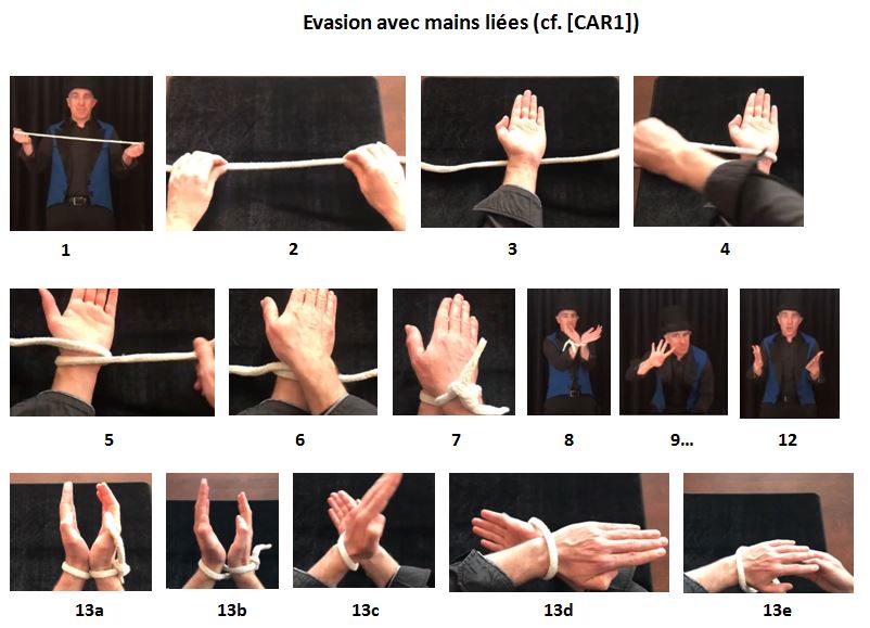
This magic trick requires only a rope approximately 70 cm long.
The steps are as follows (see Figure above, cf. [CAR1]) :
1. Place a table between you and the spectator and show a "very strong rope" stretched taut between your two hands.
2. Lay the rope on the table, parallel to the spectator.
3. Place your left hand in the middle of the rope, palm facing up.
4. Bring the right end of the rope over your left wrist, and in front of the left end.
5. Bring the left end of the rope over your right wrist, without crossing the other end.
6. Place your right hand on top of your left hand, palm facing down.
7. Ask the spectator to take the two free ends and tie them together above your hands with three tight knots.
8. Raise your arms, showing your hands tied together.
9. Lower your hands behind the table and then immediatly... raise your free right hand.
10. Lower your free hand behind the table and then immediatly... raise both hands again.
11. Repeat steps 9 to 10.
12. Lower your hands behind the table and then immediatly... raise both hands.
Explanation : Behind the table, rotate each wrist a quarter turn in the opposite direction (13a, 13b, 13C, 13d) and take the right hand out of the loop (13e). Reverse the movement to reattach both hands.
Note : a more sophisticated version of this trick exists (see [HAF]).
B6.2. Magic tricks with playing cards :
Here are some spectacular card tricks that can be done by children.
B6.2.1. The thieving Jacks :

This trick requires a 32-card deck :
1. Take three Jacks from a deck of cards and leave the deck face down on the table.
2. Tell the story : "Three thieves want to break into a house...
3. The first finds a basement window and goes through the cellar (place a Jack under the deck).
4. The second climbs onto the roof and goes through the attic (place a Jack on top of the deck).
5. The third finds an open window and goes down to the ground floor (insert a Jack into the deck)."
6. Ask the spectator to "cut" the deck.
7. Announce that the three Jacks will be together and fan out the deck to verify this.
Solution : Prepare the deck by placing a Jack (the fourth) on top. The three Jacks reunited at the trick end are not the same, but this often escapes the spectator.
B6.2.2. The four Kings :

This trick is a variant of the "Three thieves" trick. It requires a 32-card deck :
1. Fan out the four Kings in front of the spectator.
2. Stack them on top of the remaining deck.
3. Take the four top cards one by one and insert them into the deck.
4. Ask the spectator to "cut" the deck into two approximately equal parts.
5. Announce that the four Kings will be together and fan out the deck to verify this.
Solution : Before starting the trick, discreetly add a stack of four more cards under the fan of the four Kings, well hidden by the first King (see Figure above).
B6.2.3. The four Aces :

This trick requires a 32-card deck :
1. Give the spectator a deck of cards to shuffle, then take the deck back, and present it vertically, facing the spectator.
2. Ask him to take one of the Aces and place it face down against his chest.
3. Pass the deck behind your back, then show it to the spectator again, asking him to replace his Ace in the deck.
4. Give the deck back to the spectator to shuffle, then take the deck back, and remove the chosen Ace.
Solution :
- Prepare the deck by setting the "point" of each Ace in the card center in the same orientation (spades, hearts, clubs), the Ace of diamonds being symmetrical (see Figure above).
- Behind your back, turn the deck of cards halfway around (top/bottom reversed).
- The chosen Ace is the Ace of diamonds if no "point" is reversed, and the Ace with a reversed "point" otherwise.
- Warning : Remove the chosen Ace from the deck, thumb pointing towards you, then present the card to the spectator, thumb pointing towards him (this reverses the card's orientation so the trick can be repeated). Then place the card back in the deck, thumb pointing towards the spectator.
Note : In terms of face cards (Jack, Queen, King, and Joker), numbered cards (from Ace to Ten), and possible indexes placed in opposite corners, standard post-19th-century French 54-card decks generally feature cards that are symmetrical by rotating them a half turn. There are 18 exceptions : the two Jokers (red and black), the four Sevens (one for each suit), and four triplets of cards (spades, hearts, clubs) corresponding to Aces, Threes, Fives, and Nines.
B6.2.4. The found card : :
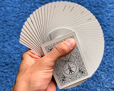
This trick is a spectacular and little-known generalization of the "Four Aces" trick. It requires a 32-card deck :
1. Give the spectator a deck of cards to shuffle, then take the deck back, and present it vertically, facing the spectator.
2. Ask him to take any card and place it face down against his chest.
3. Pass the deck behind your back, then present it to the spectator again, asking him to replace his card in the deck.
4. Give the deck back to the spectator to shuffle, then take the deck back, present it fanned out, quickly scroll through the cards one by one, and remove the chosen card.
Solution :
- Not every deck of cards has perfect printing in the center of each card. The white band separating the top edge of the card from the top of its printed portion (the short side of the rectangle surrounding each face card, or the head of each number) is not identical at the top and bottom of the card. With few exceptions, each card therefore has a small band and a large band.
- Prepare the deck by setting the small band on the same side throughout. If the band is almost identical at the top and bottom of the card, discard the card from the deck.
- Behin your back, turn the deck of cards halfway around (top/bottom reversed).
- When scrolling through the cards, aim for the top band. The chosen card is the one whose band suddenly changes size (small/large) due to a stroboscopic effect.
- Warning : Remove the chosen card from the deck, thumb pointing towards you, then present the card to the spectator, thumb pointing towards him (this reverses the card's orientation so the trick can be repeated). Then place the card back in the deck, thumb pointing towards the spectator.
B6.2.5. Magical memorization :
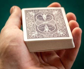
This spectacular trick requires a 32-card deck :
1. Shuffle the deck.
2. Pass the deck behind your back, move the bottom card to the top, and present the deck vertically, facing the spectator.
3. Announce the card and repeat from step 2.
4. Continue in this way with all the cards in the deck.
Solution :
- At the end of the shuffle, discreetly memorize the last card on the bottom of the deck.
- While presenting the deck to the spectator, memorize the bottom card that is facing you.
B6.2.6. The 27-card trick :

This purely mathematical trick requires a 32-card deck :
1. Make a deck of exactly 27 cards.
2. Fan out the deck to the spectator. Ask him to mentally remember a card C and then to give a number N from 1 to 27. Secretly calculate the number R = N - multiples of 9, adjusting R between 1 and 9 (examples : if N = 18, then R = 9 ; if N = 22, then R = 4).
3. Turn the deck face down and arrange the cards face up on the table in three columns of nine cards each, placing them in horizontal rows of three, from left to right and from top to bottom (see Figure above).
4. Ask the spectator to point to the column containing his card, then stack the cards, face up and column by column, picking up the designated column in the position p = R - multiples of 3, adjusting p between 1 and 3 (example: if R = 4, then p = 1). More simply, column p is immediately visible without any calculation by distributing R in a 3x3 square, in horizontal rows of 3, from left to right and from top to bottom (see Figure above).
5. Turn the deck face down again and form three columns of nine cards each again, as before, and ask for the column again. Stack the cards, face up and column by column, picking up the designated column in position q = 1 + Int[(R - 1)/3] (example : if R = 4, then q = 2). More simply, column q is immediately visible without any calculation by distributing R in a 3x3 square, in vertical columns of 3, from top to bottom and from left to right (see Figure above).
6. Turn the deck face down again and form three columns of nine cards each again, as before, and ask for the column again. Locate card C in position R of this column. Stack the cards, face up and column by column, picking up the designated column in position r = 1 + Int[(N - 1)/9] (example : if N = 22, then r = 3). More simply, column r is immediately visible without any calculation by distributing N in a 9x3 rectangle, in vertical columns of 9, from top to bottom and from left to right (see Figure above).
7. Turn the deck face down and place the cards one by one face down on the table, counting from 1. On the Nth card, announce card C and turn it face up.
Demonstration :
Let p, q and r be the order numbers (between 1 and 3) in which the designated column is picked up at each spread of the cards in three columns.
Let Np, Nq and Nr be the position in the deck (between 1 and 27) of the first card in the block containing card C, after picking up the designated column p, q or r, and reforming the deck.
At each spread, the exact position of card C in the deck is not determined, but rather the position of the first card in the block containing it. The size of this block is divided by 3 at each step.
At the first spread, the deck of 27 cards is divided into 3. After picking up column p and reforming the deck, card C is mechanically located in a continuous block of 9 cards, the position of the first card of which is :
Np = 1 + 9(p - 1), corresponding to the interval Ip = [Np, Np + 8].
Examples :
If p = 1, Ip = [1, 9].
If p = 2, Ip = [10, 18].
If p = 3, Ip = [19, 27].
At the second spread, this block of 9 cards is divided into 3. After picking up column q and reforming the deck, card C is mechanically located in a continuous block of 3 cards, the position of the first card of which is :
Nq = 9(q - 1) + 1 + (Np - 1)/3 = 1 + 9(q - 1) + 3(p - 1), corresponding to the interval Iq = [Nq, Nq + 2].
Examples :
If p = 1 and q = 1, Iq = [1, 3].
If p = 1 and q = 2, Iq = [10, 12].
If p = 2 and q = 1, Iq = [4, 6].
If p = 2 and q = 2, Iq = [13, 15]
If p = 3 and q = 1, Iq = [7, 9]
At the third spread, this block of 3 cards is divided into 3. After picking up column r and reforming the deck, card C is mechanically located in a block of only 1 card, whose position is :
Nr = 9(r - 1) + 1 + (Nq - 1)/3 = 1 + 9(r - 1) + 3(q - 1) + (p - 1), corresponding to the interval Ir = [Nr, Nr].
Examples :
If p = 1, q = 1 and r = 1, Ir = [1, 1].
If p = 1, q = 1 and r = 2, Ir = [10, 10].
If p = 1, q = 2 and r = 1, Ir = [4, 4].
If p = 1, q = 2 and r = 2, Ir = [13, 13].
If p = 2, q = 1 and r = 1, Ir = [2, 2].
If p = 2, q = 1 and r = 2, Ir = [11, 11].
If p = 2, q = 2 and r = 1, Ir = [5, 5].
If p = 2, q = 2 and r = 2, Ir = [14, 14].
If p = 3, q = 1 and r = 1, Ir = [3, 3].
Given the expression for Nr, the number N at the end of the trick satisfies the formula : N - 1 = 9(r - 1) + 3(q - 1) + (p - 1)
This trick is therefore simply a decoding of the number (N - 1) into base 3, column by column, where each column choice provides one of the three ternary digits.
Given this formula, the simplified expressions for p, q, and r are then as follows :
We set R = (N - 1) mod 9 + 1 = N - multiples of 9, adjusting R between 1 and 9
p = (N - 1) mod 3 + 1 = (R - 1) mod 3 + 1 = R - multiples of 3, adjusting p between 1 and 3 = column of the square p(R) in Figure above.
q = Ent[(N - 1)/3] mod 3 + 1 = Ent[(R - 1)/3] + 1 = column of the square q(R) in Figure above.
r = Ent[(N - 1)/9] + 1 = column of the rectangle r(N) in Figure above.
B6.2.7. The three-card monte :
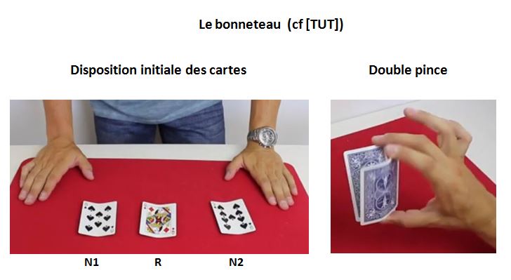
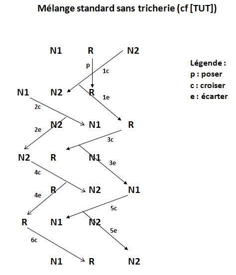
The Three-card monte (bonneteau) is a street card game where a player must locate the red card among three cards after a rapid shuffle.
Required equipment :
- A rigid tablet or thick cardboard serving as a table.
- Three cards : two black (for example, the King of spades and the King of clubs) and one red (the Queen of hearts).
- Cash for the player's bets.
The monte operator (bonneteur) is a professional manipulator who presents the game, shuffles the cards, and runs the play.
The player places a bet and points to the card they believe is the red.
The shills (barons) are the operator's accomplices. They pretend to play and win to build confidence, attract passersby, watch for police, and calm losers.
In France, three-card monte is illegal as it constitutes a game of chance played in public with money stakes (Article L. 324-1 of the Internal Security Code).
Game rules :
1. The operator shows the three cards face up and places the red between the two black cards. The cards are slightly folded lengthwise to make them easier to grip by the short edges when they are face down (see Figure 1 above [TUT]).
2. He turns over the cards, face down, and shuffles them quickly on the table with linear movements.
3. The operator turns over the middle card, which hasn't changed (red). He turns it over again and performs a second shuffle that appears identical to the first.
4. The player then places a bet and points to the card (left, center, right) they think is the red.
5. The operator reveals the chosen card. If it's the red, the player receives double their bet. Otherwise, the bet is lost.
In practice, the game is rigged :
1. The operator often starts with a few honest, slow rounds where the shills win easily to gain the public's confidence.
2. Once a real player participates, the operator alters his manipulations :
- Index rotation drop : A specific two-card grip allowing independent release of the top or bottom card. This "double pinch" technique is ideal for prolonged shuffles.
- Filage (sliding) : Discreet sliding of one card under another.
- Quick swap : Concealed swap of two cards at the moment of placement.
- Result : The operator always maintains control of the red' true position.
Index rotation drop technique [TUT] :
The index rotation drop technique consists of discreetly releasing the top card (black) while retaining the bottom card (red).
- Initial position : The top card (black) is held between thumb and index at the two corners. The bottom card (red) is held identically but between thumb and middle finger. Both cards share a common thumb pivot point, while a small wedge-shaped gap exists between their opposite edges (see Figure 2 above [TUT]).
- Execution : Turn the wrist to clearly show the red to the player, then reposition palm facing the table. During the linear movement above the table, the index performs a sharp but discreet rotation, releasing pressure on the top card (black). It slides passively forward, while thumb/middle finger firmly hold the bottom card (red).
- End of movement : The dropped card seems to follow the continuity of the shuffle and is always the bottom card.
- One-handed double drop [TUT, 04:20] :
- Initial layout of the cards on the table, as seen by the player : N1 R N2 (N = black, R = red).
- Two cards are picked up in double pinch : first N1 as top card, then R as bottom card. Turn the wrist to clearly show R to the player.
- Perform first drop of card (N1) by placing it in the middle, then the remaining card (R) to the left, secretly transforming the layout to R N1 N2.
- Pick up two other cards in double pinch : first R as top card, then N2 as bottom card. Turn the wrist to clearly show N2 to the player.
- Perform second drop of card (R) by placing it to the right, then the remaining card (N2) to the left, secretly transforming the layout to N2 N1 R.
- The player is doubly tricked, thinking R is either in the middle or to the left.
Standard shuffle technique :
The standard shuffle is performed in three rhythmic phases (see Figure 3 above and [TUT, 03:58]) :
- Phase 1 : Central drop. Place one of the two cards held in double pinch at the center using the index rotation drop technique.
- Phase 2 : Five Croiser-Ecarter sequences :
- Croiser : Pass a card over the one immediately to its left (or right).
- Ecarter : Move an outer card to the right (or left), creating a temporary empty space for another card.
- The five sequences systematically alternate sides (Left/Right) per the binary pattern : Croiser L - Ecarter R | Croiser R - Ecarter L | Croiser L - Ecarter R | Croiser R - Ecarter L | Croiser L - Ecarter R
- Phase 3 : Final Croiser. Croiser once more to the Right.
When the shuffle is executed without cheating, with a drop of the bottom (red) card, the initial N1 R N2 layout remains unchanged, reinforcing the illusion of a neutral process.
B6.3. Magic tricks with numbers :
Here are some spectacular number-based tricks.
B6.3.1. Mind readind :
[narrated by Clément Brizzard]
This spectacular trick is a magical mind-reading experiment.
The magician asks a member of the audience to think of a whole number between 1 and 100,
then multiply it by 9,
then subtract 5,
then add the digits of the resulting number,
then repeat this last operation if the result is greater than 9,
then convert the result into a letter of the alphabet : A for 1, B for 2, C for 3, etc.,
then think (in French) of a European country beginning with that letter,
then think (in French) of a fruit beginning with the last letter of the European country.
The magician then announces that the fruit thought of is a "kiwi". If the person says this is incorrect, then the magician announces that the fruit is a "kaki".
At no point did the person speak.
Explanation :
Any integer N with n digits is of the form cn...c2c1 and can be written :
N = 10n - 1 cn + ... + 100 c3 + 10 c2 + c1 = (10n - 1 - 1) cn + ... + 99 c3 + 9 c2 + (cn + ... + c3 + c2 + c1)
Therefore, N is of the form : N = 9K + sum S of the digits of N.
If S is greater than 9, then similarly : S = 9K' + sum S' of the digits of S.
In conclusion, every number N is always the sum of a multiple of 9 and a remainder between 1 and 9 corresponding to the simple or repeated sum of the digits of the number N.
Example 1 : 8 = 9 x 0 + 8, where 8 is the digit of the number 8.
Example 2 : 34 = 9 x 3 + 7, where 7 is the sum 3 + 4 of the digits of the number 34.
Example 3 : 38 = 9 x 4 + 2, where 2 is the sum 3 + 8 = 11 of the digits of 38, and then the sum 1 + 1 of the digits of 11.
If N is already a multiple of 9 (as requested by the magician), then this remainder is necessarily 9.
Subtract 5 from this N, which is a multiple of 9, so the remainder is 4.
The only European country beginning with the letter D (corresponding to 4 in the alphabet) is "Danemark" (in French).
The only common fruits beginning with a K (corresponding to the last letter of the word "Danemark") are "kiwi" and "kaki" (in French).
Hence the magician's answer, without any mind reading.
Improved solutions :
- Offer to choose N between 1 and 10 rather than between 1 and 100.
- Multiply N by 10 and then subtract N, rather than multiplying N by 9.
- We can repeat the trick a second time, but with a different person, and with the following modification : Instead of asking for a European country, ask directly for a fruit whose name begins with the letter of the alphabet (which gives the "Datte" corresponding to the result 4 = D).
-
We can repeat the trick a third time with any person, asking them to subtract 7 instead of 5. Then, instead of asking for a European country, ask directly for a fruit whose name begins with the letter of the alphabet (which gives the "Banane" corresponding to the result 2 = B).
B6.3.2. The age of children :
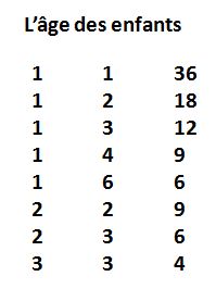
A father is talking to the mail carrier : "I have three children. The product of their ages is equal to 36. The sum of their ages is equal to the number of the house across the street."
The mail carrier looks at this number and asks : "I'm missing one piece of information to solve the problem.
"
The father replies : "That's right. My oldest is blond."
The mail carrier then gives the solution. How did he do it ?
Solution to this riddle :
36 can be obtained in 8 different ways :
1 x 1 x 36, which adds up to 38
1 x 3 x 12, which adds up to 16
1 x 4 x 9, which adds up to 14
1 x 6 x 6, which adds up to 13
2 x 2 x 9, which adds up to 13
2 x 3 x 6, which adds up to 11
3 x 3 x 4, which adds up to 10
Since the mail carrier couldn't determine the sum by looking at the house number, this indicates that the sum has several possibilities, not just one.
Only 13 is ambiguous, and since there's only one eldest child, the children are therefore 2, 2, and 9 years old.
B6.3.3. The Maurice Dagbert's trick :

[Heard on the radio in the 1980s]
A famous French calculating prodigy, Maurice Dagbert, presented this seemingly impossible problem :
"Choose an integer between 1000 and 3000 [2139 was given]. I will now calculate two lists of 17 integers each, such that :
- The sums of the numbers are equal to 2139,
- The sums of the squares of the numbers are equal,
- The sums of the cubes of the numbers are equal,
and so on up to the sixth power of the numbers.
Furthermore, all numbers will be different from each other, whether within a list or between lists."
For the number N = 2139 chosen, he then stated, after only a few minutes, the following two lists :
First list (La) = [ 59, 63, 68, 82, 86, 100, 105, 109, 139, 143, 148, 156, 162, 173, 175, 185, 186 ]
Second list (Lb) = [ 60, 61, 70, 79, 89, 98, 107, 108, 140, 141, 151, 153, 164, 170, 178, 183, 187 ]
A computer confirmed the calculations.
The explanation is as follows :
1. Mathematical modeling :
The problem can be written as the following system of equations S, with k = 6, n = 17, and Sum = N.
(1) System S :
∑iai = ∑ibi = Sum
∑iai2 = ∑ibi2
∑iai3 = ∑ibi3
...
∑iaik = ∑ibik
where :
i = index from 1 to n
n = size of each list
k = power of the termes of last equation
Sum = sum of the terms of first equation
ai and bi = positive integers, all distinct
2. First tip :
Each list of 17 numbers is actually a concatenation of two sublists of 8 and 9 numbers each, satisfying the following subsystems S1 and S2 :
(21) Subsystem S1 = System S for k = 6, n = 8 and Sum = N1, corresponding to the following partial lists :
L1a = [ 59, 63, 68, 82, 86, 100, 105, 109 ]
L1b = [ 60, 61, 70, 79, 89, 98, 107, 108 ]
(22) Subsystem S2 = System S for k = 6, n = 9 and Sum = N1, corresponding to the following partial lists :
L2a = [ 139, 143, 148, 156, 162, 173, 175, 185, 186 ]
L2b = [ 140, 141, 151, 153, 164, 170, 178, 183, 187 ]
(23) Additional condition : N1 + N2 = N
3. Second tip :
Each of these subsystems is known in mathematics as the "PTE (or Prouhet-Tarry-Escott) Problem" [WIK1].
This problem has the remarkable property of being invariant under translation of variables [WIK1]. If we replace the variables ai and bi respectively with (a*i = α ai - β) and (b*i = α bi - β), where α and β are any two constants, then the new variables are solutions to the same problem by simply changing Sum to Sum* = (α Sum - n β).
This translation allows us to normalize the solutions, for example, by requiring that they be positive and that zero be included.
For S1, if we choose α1 = 1 and β1 = 84, we obtain the translated subsystem S1* as follows :
(31) Subsystem S1* = subsystem S1 of sum N1* = N1 - 8 β1, corresponding to the following translated lists :
L1a* = [ -25, -21, -16, -2, 2, 16, 21, 25 ]
L1b* = [ -24, -23, -14, -5, 5, 14, 23, 24 ]
This solution, called even-sized and symmetric [WIK1], is of the form [ -c4, -c3, -c2, -c1, c1, c2, c3, c4 ] for the first list and [ -d4, -d3, -d2, -d1, d1, d2, d3, d4 ] for the second.
This symmetry automatically makes equations in odd powers valid in subsystem S1*, which can be simplified to :
Subsystem S1* :
n = 4
∑ici2 = ∑idi2
∑ici4 = ∑idi4
∑ici6 = ∑idi6
corresponding to the following basic lists :
C1 = [ ci ] = [ 2, 16, 21, 25 ]
D1 = [ di ] = [ 5, 14, 23, 24 ]
For S2, if we choose α2 = 1 and β2 = 163, we obtain the translated subsystem S2* as follows :
(32) Subsystem S2* = subsystem S2 of sum N2* = N2 - 9 β2, corresponding to the following translated lists :
L2a* = [ -24, -20, -15, -7, -1, 10, 12, 22, 23 ]
L2b* = [ -23, -22, -12, -10, 1, 7, 15, 20, 24 ]
This solution, called odd-sized and symmetric [WIK1], is of the form [ -c5, -c4, -c3, -c2, -c1, d2, d3, d4, d5 ] for the first list and [ -d5, -d4, -d3, -d2, c1, c2, c3, c4, c5 ] for the second.
This symmetry automatically makes equations in even powers valid in subsystem S2*, which can be simplified to :
Subsystem S2* :
n = 5
∑ici = ∑idi
∑ici3 = ∑idi3
∑ici5 = ∑idi5
with d1 fictitious = 0
corresponding to the following basic lists :
C2 = [ ci ] = [ 1, 7, 15, 20, 24 ]
D2 = [ di ] = [ 0, 10, 12, 22, 23 ]
Furthermore, the symmetry of the solutions, for each subsystem S1* and S2*, makes the sums N1* and N2* zero, which can be written :
(33) N1 = 8 β1 and N2 = 9 β2
Given relation (23), this gives the following necessary condition :
(34) N = 8 β1 + 9 β2
Note that this condition is always attainable, since 8 and 9 are coprime.
4. Choice of a solution for subsystem S1* :
Subsystem S1* (see relations (31)) is that of the PTE problem of size n = 4 and specific powers k = 2, 4, and 6.
Several solutions have been known since 1913, including the following [SHU1] :
[ 2, 16, 21, 25 ] = [ 5, 14, 23, 24 ]
[ 7, 24, 25, 34 ] = [ 14, 15, 31, 32 ]
[ 7, 31, 36, 50 ] = [ 18, 20, 41, 49 ]
[ 9, 47, 49, 67 ] = [ 23, 31, 61, 63 ]
The first solution is the smallest solution in non-negative integers for these three powers [SHU2].
It is highly probable that Maurice Dagbert knew these solutions and used the first one.
5. Choice of a solution for subsystem S2* :
The S2* subsystem (see relations (32)) corresponds to the PTE problem of size n = 5 and specific powers k = 1, 3, and 5.
While published solutions are scarce, they can be found analytically. The approach involves pairing elements from the two lists and then solving the resulting quadratic system using an appropriate method, such as that by elimination of variables.
Both approaches rely on the analytical solution of an underdetermined quadratic system of rank 2 with 5 variables, producing a family of real solutions, complemented by a short phase of targeted successive trials aimed at achieving integer values that exactly satisfy the equations.
The steps are as follows :
1. We arbitrarily fix 5 small integer values δi (for example, between -3 and 3) such that ∑i[δi] = 0 with δi = ci - di
2. We set xi = mi2 with mi = (ci + di)/2 corresponding to the local center of the variables ci and di, which induces : xi # ci2 # di2 # ci di
where the symbol "#" means "very little different"
3. Given the identities : (c3 - d3) = (c - d)(c2 + c d + d2) and (c5 - d5) = (c - d)(c4 + c3 d + c2 d2 + c d3 + d4), equations S2b become :
∑ici - ∑idi = ∑i[δi] = 0
(∑ici3 - ∑idi3 # 3 ∑i[δi xi]) = 0
(∑ici5 - ∑idi5 # 5 ∑i[δi xi2]) = 0
4. Using one of the methods mentioned above, we solve the following quadratic system :
(50) (∑i[δi xi] = 0) and (∑i[δi xi2] = 0)
which gives a family of real solutions for xi.
Solution by elimination of variables :
We fix 3 free variables, for example x1, x2 and x3
We then eliminate x4 between the two equations, which gives an equation of the form : A x52 + B x5 + C = 0, where A, B, and C are explicit quadratic polynomials in x1, x2 and x3, as follows :
A = δ5 (δ4 + δ5)
B = 2 δ5 P
C = P2 + δ4 Q
with P = ∑i=1,3[δi mi2] and Q = ∑i=1,3[δi mi4]
We find the real solutions x5 = [-B ± √(B2 - 4 A C)]/(2 A) and x4 obtained from the equation (∑i[δi xi] = 0).
5. We look for xi close to the square of an integer or a half-integer, which gives ci = √xi + δi/2 and di = √xi - δi/2
6. We substitute the integer solutions ci and di into the exact equations (32) for verification.
7. If the initial result is not verified, further tests are performed by modifying the parameters at two possible levels :
- Exploration of the 3 free parameters xi.
- Selection of the deviation vector δi.
It is highly probable that Maurice Dagbert himself obtained the basic lists (32) using this simple method.
Example of a complete calculation using the variable elimination method :
For example, we fix the first three numbers ci to 1, 7, and 15, and their corresponding values di to 0, 10, and 12.
This is equivalent to fixing the first three values of δi and xi.
We also set (first attempt) the values of δ4 = -2 and δ5 = 1.
We then seek to calculate the last two numbers c4 and c5, and their corresponding values di and di.
The calculations give : P = 330.25, Q = 83985.06, A = -1, B = 2 P, C = P2 - 2 Q, (B2 - 4 A C) = 447.932
Hence :
x5 = 10.312 or 23.542
We retain x5 = 23.542, close to the square of a half-integer (since δ5/2 = 1/2).
c5 = √x5 + δ5/2 = 24.04
d5 = √x5 - δ5/2 = 23.04
x4 = -(δ5 x5 + P)/δ4 = 21.032
We retain x4 = 21.032, close to the square of an integer (since δ4/2 = -1).
c4 = √x4 + δ4/2 = 20.03
d4 = √x4 - δ4/2 = 22.03
We substitute the integer solutions c5 = 24, d5 = 23, c4 = 20, d4 = 22, into the exact equations (32), which are found to be verified on this first trial.
6. Calculation of β1 and β2 from a given N :
Relation (34) is a Diophantine equation that can be written more simply as :
(60) β1 = 9 u - N and β2 = N - 8 u, with u arbitrary
But three additional constraints must be met :
1. The partial lists of S1 and S2 must be joined to give the illusion of two unique and increasing lists of 17 numbers each.
2. These partial lists must not contain duplicates.
Given translated lists (31)(32), these two constraints can be written :
(β2 + Min[L2a*, L2b*]) greater than and close to (β1 + Max[L1a*, L1b*])
with Min[L2a*, L2b*] = -24 and Max[L1a*, L1b*] = 25
Given relations (60), this can be written :
(61) u smaller than and close to u max
with u max = (2 N - (Max[L1a*, L1b*] - Min[L2a*, L2b*]))/17 = (2 N - 49)/17
For N = 2139, u max = 248.8
3. All numbers in lists (La) and (Lb)
must be greater than zero.
Given the translated lists (31)(32), this can be written :
β1 + Min[L2a*, L2b*] > 0
Given relation (60), this can be written :
(62) u > u min
with u min = (N - Min[L2a*, L2b*])/9 = (N + 24)/9
For N = 2139, u min = 240.3
Given conditions (61)(62), Maurice Dagbert chose 247 for the value of u, resulting in values of 84 and 163 for β1 and β2.
It remains to be ensured that umin < umax for any value of N.
Given conditions (61)(62), this introduces a new constraint :
(63) N > (9 Max[L1a*, L1b*] - 26 Min[L2a*, L2b*] = 849)
Maurice Dagbert imposed 1000 as the minimum value of N to satisfy this constraint, which then avoids calculating u min.
7. No duplicates in a list or between lists of 17 numbers :
This remarkable property results from three observations :
- By construction, the elementary lists C1 and D1 (see relations (31)) have no duplicates, either internally or between themselves. Therefore, the same is true for the translated lists L1a* and L1b*, given their symmetries, as well as partial listes L1a and L1b.
- Also by construction, the elementary lists C2 and D2 (see relations (32)) have this same property. Therefore, the same is true for the translated lists L2a* and L2b*, given their symmetries, as well as partial listes L2a and L2b.
- By previous choice (see relation (61)), the partial lists L1a and L1b are disjoint from the partial lists L2a and L2b.
Consequently, the two lists of 17 numbers cannot have duplicates, either internally or between themselves, since they result from the simple concatenation of L1a and L2a for the first and of L1b and L2b for the second.
8. Construction of the lists of 17 numbers :
The two lists of 17 numbers provided by Maurice Dagbert are then compiled in four steps :
1. Calculation of u according to relations (61)(62).
2. Calculation of β1 and β2 according to relations (60).
3. Memorization of three lists of gaps based on the gaps between consecutive numbers in each translated list L1a*, L1b*, L2a*, L2b* (see relations (31)(32)) :
List of gaps E1 = [ 4, 5, 14, 4, 14, 5, 4]
List of gaps E2 = [ 4, 5, 8, 6, 11, 2, 10, 1 ]
List of gaps E3 = [ 1, 9, 9, 10, 9, 9, 1 ]
4. Construction of two lists (La) and (Lb) of 17 numbers based on these lists of gaps and the translations β1 and β2, according to the following distribution :
La = [L1a, L2a]
Lb = [L1b, L2b]
with :
L1a = [ (β1 - 25), +E1 ] composed of 8 terms
L2a = [ (β2 - 24), +E2 ] composed of 9 terms
L1b = [ (β1 - 24), +E3 ] composed of 8 terms
L2b = [ (β2 - 23), +E2! ] composed of 9 terms
The symbol "!" means that the list must be read in reverse.
Note : There is another (more complicated) way to construct the two lists of 17 numbers, based on memorizing the elementary lists C1, D1, C2, D2 (see relations (31)(32)) :
L1a = [ (β1 - C1!)4, (β1 + C1)4 ]
L2a = [ (β2 - C2!)5, (β2 + D2 )4 ]
L1b = [ (β1 - D1!)4, (β1 + D1)4 ]
L2b = [ (β2 - D2 !)4, (β2 + C2)5 ]
The symbol "!" means that the list must be read in reverse.
The symbol " " means that the fictitious term 0 in the list should be ignored.
The subscript at the bottom indicates, as a reminder, the number of terms in the quantity within the parentheses.
No duplicates in a list or between lists of 17 numbers :
This remarkable property results from three observations :
- By construction, the basic lists C1 and D1 have no duplicates, either internally or between themselves. Therefore, the same is true for the translated lists L1a* and L1b*, given their symmetries.
- Also by construction, the basic lists C2 and D2 have this same property. Therefore, the same is true for the translated lists L2a* and L2b*, given their symmetries.
- By deliberate choice, lists L1a and L2a are disjoint from lists L1b and L2b (see condition (50)).
Consequently, the two lists of 17 numbers cannot have any duplicates, either internally or between themselves, since they result from the simple concatenation of L1a and L2a for the first and of L1b and L2b for the second.
B6.4. Sources relating to Magic tricks :
[ASH] ashmarlow52, Learn This Viral Battery Trick (Youtube, 01:07).
[CAR1] Carrefour francophone, Cours de Magie avec Magislain - Tour 4 : Evasion (Youtube, 03:16).
[CAR2] Carrefour francophone, Cours de magie avec Magislain - Tour 2 : L'élastique à travers les doigts (Youtube, 03:21).
[EIT] Joseph Eitel, The Handcuff Escape Puzzle.
[GAR] Nasr Garouachi, Cordes - Playlist.
[HAF] Nadjib Haffaf, Echapper à la corde facile - DIDACTICIEL (Youtube, 02:45).
[JER] Jérémie-L'école de la magie, 3 TOURS DE MAGIE AVEC 1 ELASTIQUE (Youtube, 08:20).
[MAGE] MagieExpliquée, Apprenez la Téléportation avec un simple Elastique - Secret Révélé (Youtube, 06:43).
[MIR] Minute Facile, Régis le magicien vous explique son incroyable tour de magie avec une corde (Youtube, 03:50).
[PAU] Paulo magie, apprenez un tour impressionnant avec 2 élastiques (Youtube, 05:26).
[PRA] pratiqueTV, Tour de passe passe avec des piles (Youtube, 01:50).
[SHU1] Chen Shuwen, Non-negative Integer Solutions of a1k + a2k + a3k+ a4k = b1k + b2k + b3k + b4k ( k = 2, 4, 6 ).
[SHU2] Chen Shuwen, On the Generalization of the Prouhet-Tarry-Escott Problem.
[TUT] TUTO MAGIE, ARNAQUE OU MAGIE ? COMMENT GAGNER DE L'ARGENT AVEC 3 CARTES EXPLICATION (Youtube, 06:24).
[VAL] TUTUR VAL, 5 TOURS DE MAGIE AVEC DES ELASTIQUES (Youtube, 07:49).
[WIK1] Problème de Prouhet-Tarry-Escott.
Here is an introduction to strategy games.
This collection brings together single-player and multiplayer games for which a strategy is known : either a winning strategy for one of the two players, an optimal strategy, or simply a rational one.
Contents :
B7.1. Pawn games :
The following pawn games all have a winning strategy for one of the two players.
B7.1.1. 17 matches game :
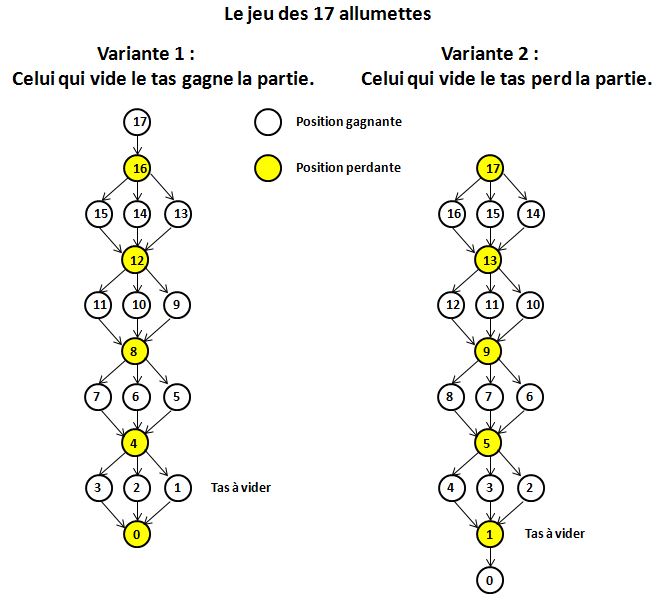
17 matches game is a two-player strategy game with a winning strategy depending on the chosen variant.
Rules of the game :
Two players face a pile of 17 matches.
Players take turns, each removing 1, 2, or 3 matches.
Two variants then exist :
V1. The player who empties the pile wins the game.
V2. The player who empties the pile loses the game.
Winning strategy :
V1 : the first player wins by always returning the game to a multiple of 4 matches (i.e., 16, 12, 8, 4, 0).
V2 : the second player wins by always returning the game to a multiple of 4 + 1 matches (i.e., 13, 9, 5, 1).
Explanation :
The game can be represented by a directed graph (called options graph), where each vertex corresponds to a game position n (number of matches remaining) and each edge corresponds to a possible move (going from position n to n - 1, n - 2, or n - 3). See Figure above.
Two types of positions are distinguished :
- A winning position (G in white) when there exists at least one move leading to a losing position (P in yellow).
- A losing position (P) when all possible moves lead to winning positions (G).
Variant V1 :
Position 0 is losing for the player whose turn it is (they cannot move and have lost).
By working backwards through the graph, we observe that :
- 1, 2, and 3 are winning,
- 4 is losing,
- then, by induction, all multiples of 4 are losing positions.
These losing positions correspond exactly to those with Grundy number (denoted 'mex') equal to zero (since it is an impartial game), which explains why the player who can identify them can always force a win.
Variant V2 :
Position 0 is winning for the player whose turn it is (they win without moving since the opponent took the last match).
By working backwards through the graph, we observe that :
- 1 is losing,
- 2, 3, and 4 are winning,
- then, by induction, all positions of the form 4 k + 1 are losing (with k a non-negative integer).
Here too, these losing positions are exactly those with Grundy number zero, explaining the periodicity modulo 4.
Grundy number :
In an impartial game (like the 17 matches game), the Grundy number g(n) of any position n is defined as the mex (minimum excludant) of the Grundy numbers of its positions reachable in one move, where mex denotes the smallest natural integer absent from the set.
Any position with no possible moves also has a Grundy number equal to 0.
Applied to the 17 matches game, this leads to the following recurrence relation :
g(n) = mex{g(n - 1), g(n - 2), g(n - 3)} pour n ≥ 1
Variant V1 :
g(0) = 0 since no move is possible from position 0, hence the result : g(n) = n mod 4
Variant V2 :
g(1) = 0, hence the result : g(n) = (n - 1) mod 4
Interpretation : Positions with Grundy number zero are exactly the losing positions. The winning strategy therefore consists of always moving to return the opponent to a zero-Grundy position.
B7.1.2. Heap game :

Heap game, also known as Nim or Marienbad game, is a winning strategy game for two players based on simple and fascinating mathematical principles.
Rules of the game :
Two players are presented with several heaps of objects (stones, cards, matches, scallop shells). The number of heaps and the number of objects per heap are arbitrary.
Players take turns, and each player removes as many objects as they wish (but at least one) from a single heap.
The player who empties the last heap wins the game.
Winning Strategy :
The winning method relies on a specific addition operation called "Nim_addition". We calculate the XOR sum of the heap sizes written in binary notation (that is, bitwise "exclusive OR", where the result bit is 1 if and only if the bits are different).
If this Nim_addition is zero, the position is a losing one (called an "even" position). Otherwise, the position is a winning one ("odd" position), and there is always at least one action that can bring the Nim_addition back to zero.
Example (see Figure above) : Consider three heaps of size 3 (011 in binary), 4 (100 in binary), and 5 (101 in binary). The Nim_addition (denoted "⊕") is : 3 ⊕ 4 ⊕ 5 = 2 (10 in binary), which is not zero. The first player can therefore win by adjusting the size of one of the heaps.
A more visual way to do this is as follows [DEL1]. We decompose each size into sub-heaps pi, each containing i objects, where i is a power of 2. This is equivalent to writing these sizes in binary notation.
For each power of 2, we count the total number of corresponding sub-heaps. A position is considered a losing position if this number is even for all powers of 2.
In the previous example, we have : 3 = p2 + p1 ; 4 = p4 ; 5 = p4 + p1. Here, the sub-heap p2 appears only once. To restore an even position, we must therefore remove this sub-heap, which reduces the heap of size 3 to 1.
Explanation :
Let n heaps be given, with ti being the size of heap i. The Nim_addition is : S = t1 ⊕ ... ⊕ ti ⊕ ... ⊕ tn
A legal move consists of choosing a heap m and modifying its size tm by a strictly smaller integer t'm, the other heaps remaining unchanged.
The initial Nim_addition S is then written : S = t1 ⊕ ... ⊕ tm ⊕ ... ⊕ tn
After the move, it becomes : S' = t1 ⊕ ... ⊕ t'm ⊕ ... ⊕ tn
Given the identity : tm ⊕ tm = 0, and the commutativity and associativity of the XOR operator, this can also be written :
(*) S' = S ⊕ (tm ⊕ t'm)
1. Case S = 0 : An even position always leads to an odd position.
Given relation (*), if S = 0, then we have : S' = tm ⊕ t'm
Since tm ≠ t'm, we necessarily have : tm ⊕ t'm ≠ 0, therefore S' ≠ 0.
.
The new position is thus odd.
2. Case S ≠ 0 : Starting from an odd position, there is at least one action leading to an even position.
If S ≠ 0, let r max be the rank of the most significant non-zero bit in S. In the previous example (S = 10 in binary), r max corresponds to the second rank from the right.
Therefore, there exists at least one heap m whose size tm has a bit equal to 1 at rank r max.
We then define a new size t'm = tm ⊕ S
At rank r max, there is a 1 in tm and a 1 in S, so the bit at rank r max becomes 0 in t'm. Furthermore, no higher-ranking bits are modified. We therefore have : t'm < tm, and this action allows us to play a legal move by reducing the size of the heap tm.
The relation (*) can then be written :
S' = S ⊕ (tm ⊕ (tm ⊕ S)) = (S ⊕ S) ⊕ (tm ⊕ tm) = 0
The new position is therefore even.
B7.1.3. Moore's Nim :
A generalization of the heap game, called Moore's Nim, is defined as follows [DEL1] :
Rules of the game :
On each turn, the player chooses between 1 and k distinct heaps (k fixed, example : k = 2) and removes at least one object from each of the chosen heaps.
Winning Strategy :
The method involves writing the size of each heap in binary (as in the heap game), then calculating a "Moore_addition" which is the vector obtained by adding the bits of each heap column by column modulo (k + 1).
The position is even (and losing) if all columns result in a remainder of zero, and odd (and winning) otherwise.
Example (see Figure above) : Suppose k is fixed at 2 and there are three heaps of size 3 (11 in binary), 4 (100 in binary), and 5 (101 in binary). The Moore_addition (denoted "⊕") is 3 ⊕ 4 ⊕ 5 = vector 212, which is not zero. The first player can therefore win by adjusting the size of one or two heaps, for example by removing 1 object from the heap of 4 and 2 objects from the heap of 5. The position then becomes : 3 ⊕ 3 ⊕ 3 = 0 which becomes even for the other player.
Explanation :
Let n heaps be defined, with ti = size of heap i, and k a fixed integer between 2 and n. The Moore_addition is : S = {c1, c2, ..., cr, ...} with cr = (number of heaps whose bit at rank r is 1) mod (k + 1)
1. Case S = 0 : An even position always leads to an odd position.
If S = 0, then for any rank r, the number cr of 1 bits is divisible by k + 1, which can be written as : cr = 0 mod (k + 1).
Let r max be the largest rank actually modified among the heaps chosen by the player. In this column, only the modified heaps can change bits. Since the player can modify at most k heaps, cr max varies by an integer with an absolute value at most equal to k.
Since no non-zero variation with an absolute value at most equal to k is divisible by (k + 1), divisibility by (k + 1) in this column is broken.
The new position is therefore odd.
2. Case S ≠ 0 : Starting from an odd position, there is at least one action leading to an even position.
If S ≠0, let r max be the rank of the most significant non-zero bit of S.
Let T be the set of heaps k whose size tk has a bit equal to 1 at rank r max.
Among these heaps, we can then choose a subset T' of 1 to k heaps such that, if we flip the bit at rank r max in each of the heaps of T' from 1 to 0 (by appropriately reducing these heaps), the new number of 1s in this column becomes a multiple of (k + 1).
We then proceed by descending induction on the ranks : for each rank r < r max, we adjust the same heaps (always by reducing them) so that the column r also becomes a multiple of (k + 1), without ever modifying the bits at strictly higher ranks that have already been fixed.
At each step, we act on at most k heaps, so this local correction is always possible, just as we "correct" the columns one by one in the heap set (k = 1) with the XOR operator.
At the end of this process, all columns have a number of bits set to 1 that is divisible by (k + 1).
The new position is therefore even.
Using the three heaps as the previous example (with k fixed at 2), the column-by-column correction process is as follows :
- The three heaps ti can be written in binary as follows :
t1 = 3 = 011
t2 = 4 = 100
t3 = 5 = 101
- Moore_addition gives S = 212, which is not zero (odd position).
- The maximum column r is 2 with T = {t2, t3}
- We can act on at most k = 2 heaps;. Here, these 2 heaps are sufficient with T' = T
- To make the second column a multiple of 3, we must remove the 1s from these two heaps.
One approach is to target the position {ti} = {3, 3, 3}, the only possible solution with k = 2.
We leave heap 1 unchanged, reduce heap 2 by 1 object, and heap 3 by 2 objects.
Note : For k = 3, there are several solutions leading to the positions {ti} = {3, 3, 3}, {2, 2, 2}, or {1, 1, 1}, respectively.
B7.1.4. Camel game :
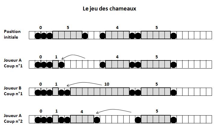
The camel game, or "ten-franc coins" game, or "push-shell" game, is a variant of the heap game, defined as follows :
Rules of the game :
The game is played on a row of squares consisting of a starting square and several coins, one per square, initially placed at arbitrary distances between coins (see Figure above).
The number of coins must be even. In the odd case, a dummy coin must be added, placed just before the starting square.
Players take turns, each moving a single coin towards the starting square, one or more squares further, without jumping over the coin already in place.
This way of moving is analogous to a caravan of camels in single file across the desert, each animal following the other without being able to overtake it.
The game ends when all the coins are blocked.
The player who makes the last move wins the game.
Winning Strategy :
The winning strategy is to play like in the heap game, maintaining a position with zero Nim_addition, and, when a move modifies this reading by increasing a heap, to immediately make a restoration move to return to an Nim_equivalent position.
The methode is as follows [TRI1] :
1. The initial position is fixed. See the example in Figure above "Position initiale" = 0111000001001000011000001, with the starting square on the left, 0 representing a free square and 1 a square occupied by a coin.
2. Starting with the coin furthest from the starting square, form disjoint pairs of successive coins from the furthest square from the starting square, each coin belonging to only one pair, and then count the number of free squares within each pair.
This counting is equivalent to defining a set of heaps of objects. See Figure above "Position initiale" showing the configuration (0, 5, 4, 5) of these heaps.
3. Next, moving a coin along the row of squares is equivalent to removing as many objects as desired from one heap among several, the winner being the one who empties the last heap.
This rule of the game is exactly the same as that of heap game, and the goal is to reach a winning even position. See Figure above "Joueur A - Coup n 1" = 0111010000001000011000001, showing the move that leads to the winning configuration (0, 1, 4, 5) corresponding to the Nim_addition 0 + 1 + 4 + (4 + 1) = 0.
4. However, unlike the heap game, a move can increase the size of a heap.
See Figure above "Joueur B - Coup n 1" = 0111011000000000011000001, showing such a move resulting in the configuration (0, 1, 10, 5).
5. To return to an "equivalent Nim" position, it is necessary to cancel any move by the opponent that would increase the size of one of the heaps. To do this, the size of the heap must be reduced to its initial value.
See Figure above "Joueur A - Coup n 2" = 0111011000010000001000001, showing the move allowing a return to the previous winning configuration (0, 1, 4, 5).
B7.2. Checkerboard games :
The following games are played on a standard 8 8 chessboard or on a 10 10 International Draughts.
B7.2.1. Northcott's game :
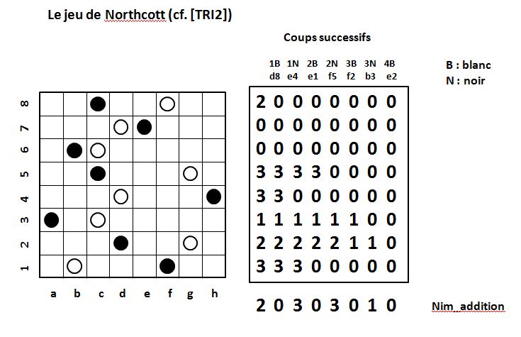
Northcott's game, invented by the American mathematician D.G. Northcott, is a variant of the heap game and camel game, defined as follows :
The rules of the game are as follows :
Initial setup :
The game is played on a standard 8x8 chessboard, with each player having 8 pawns, white for one player and black for the other (see Figure above).
The players place their pawns on the squares of the chessboard, one of each color per rank, without them occupying the same square. Thus, on each of the 8 ranks, there is one black pawn and one white pawn.
Objective :
The players take turns.
Each player chooses one of their pawns and moves it horizontally along their rank, any number of squares to the right or left, without jumping over the opponent's pawn.
The player who makes the last move wins the game.
In the original version, the game ends as soon as all the pawns are adjacent (even in the center of the ranks).
The edge-blocked variant extends the game until all the pawns are completely blocked at the edges of the chessboard. This rule makes the game more symmetrical and visually appealing.
Winning Strategy :
The method is exactly the same as in the heap game. Each rank corresponds to a heap whose size is the number of free squares between the two pawns (white and black) in that rank.
The optimal strategy is therefore to calculate the Nim_addition of these 8 values.
However, as in the camel game, the player can increase the size of a heap (by moving their pawn back), which does not change the strategy, as the situation can be restored on the next turn.
Example (see Figure above, cf [TRI2]) :
1. The initial configuration of the heaps is given by the first column of the table in the Figure. It is (2, 0, 0, 3, 3, 1, 2, 3) whose Nim_addition is 1 ⊕ 3 = 2 ≠ 0.
2. Assume that the white pawns belong to the winning player. To give their opponent an even position, this player must subtract 2 from one of the ranks, for example by moving their white pawn to position d8, leaving a configuration (0, 0, 0, 3, 3, 1, 2, 3) whose Nim_addition is 0 (see Figure above).
3. The subsequent moves for both players are given in the table of the Figure.
4. If the white and black pawns are all facing each other, but not all blocked against the edges of the chessboard, the player forced to move (Black) can only move one of the pawns back, increasing the number of free squares between the pawns, which the other player (White) immediately reduces to 0.
5. The game therefore ends in favor of the initially winning player (White), whether in the original version of the game or the edge-blocked variant.
B7.2.2. Wolf and Sheep :
Wolf and Sheep is a winning strategy game for two players.
The rules of the game are as follows :
Initial setup :
The game of Wolf and Sheep is played on a 10 x 10 International Checkers board, oriented with a white square in the bottom right corner, and using only the white squares.
At the start of the game, the wolf (black pawn) is placed on one of the white squares on one edge of the board, chosen by the player controlling it.
The 5 sheeps (white pawns) are placed in a line on the 5 white squares on the opposite edge.
Objective :
Players take turns.
The wolf starts the game. Its objective is to cross the line formed by the sheeps and reach the opposite edge of the board, which is initially occupied by the sheeps.
The sheeps win if they manage to completely block the wolf.
Movement rules :
The wolf moves one square diagonally, either forward or backward.
The sheeps also move one square diagonally, but only forward.
Capture rules :
There is no capturing or jumping.
Winning Strategy :
The strategy is successful for the sheeps in about 25 moves if they flawlessly follow these rules [PER][CHA] :
1. Advance without pursuing : The sheeps must never try to encircle the wolf or advance toward its position. The goal is to gradually reduce the wolf's room for maneuver, never to attack.
2. Advance in a compact line : The sheeps must remain aligned in a single rank or two adjacent ranks, without making isolated advances, so as never to create an exploitable gap.
3. Block the wolf's two possible moves : The sheeps must first occupy the two squares diagonally directly in front of the wolf.
4. Only play useful moves : The sheeps must only make moves that directly contribute to respecting the three previous rules.
5. Final blockade : When the wolf is trapped against an edge or in a corner of the board, the sheeps can break the compact line to occupy all accessible adjacent diagonal squares.
B7.2.3. International Draughts :
The rules of the game are as follows [PER][CHA] :
Initial setup :
International Draughts is played on a 10 x 10 board, oriented with a white square in the bottom right corner, and using only the black squares.
At the start of the game, 20 white and 20 black men are placed on the first four ranks on each side of the players.
Objective :
Players take turns.
White always moves first.
A player wins if the opponent has no more pieces or cannot move.
The game is declared a draw if :
- No player can advance towards a capture (for example, when the game only involves movable Kings, with no possibility of capture),
- The same position is repeated three times with the same player moving and the same movement options,
- 25 consecutive moves are played without a capture or King promotion.
Movement rules :
- Men move one square diagonally forward if the square is empty.
- A King can move diagonally any number of squares, forward or backward, as long as the square is empty.
Capture rules :
- A piece (man or King) can jump forward or backward over one or more opponent's pieces in a single turn, but cannot jump over the same piece more than once.
- Each opponent's piece that is jumped over is captured and removed from the board at the end of the complete sequence of captures.
- If a piece can capture, it must do so. If multiple capture sequences are possible (multiple jump), the player must choose the one that captures the most pieces.
Special rules :
- A man is promoted to a King when it reaches the last opponent's rank, symbolized by the stacking of a second man.
- Touch-play : A touched piece must be played, unless announcing "adjust" (adjusting its position) before touching the piece.
Winning Strategy :
There is no known winning strategy in International Draughts.
The optimal strategy is to minimize gross errors by following these rules [PER][CHA] :
1. Advance as a unit : Men in tandem or groups of 2 or 3 protect each other and make it harder for the opponent to capture.
2. Protect with a pyramid formation : When advancing a piece, ensure that two other pieces diagonally behind it protect it.
3. Play in the center first : The wings are difficult to defend and easy to block.
4. Simplify the game : Force simple exchanges (1 for 1) as soon as possible, provided you maintain a compact position. Fewer pieces mean fewer potential traps.
5. Detect open diagonals : When long open diagonals exist, check that the opponent cannot exploit them to place a King or launch a multiple jump, while simultaneously exploiting them offensively yourself.
6. Anticipate multiple jumps : Check before playing that the move doesn't involve an opponent's multiple jump.
7. Secure any King promotion : Before attempting a promotion, check that the destination square doesn't allow for an immediate capture.
8. Crown early : Aim to promote one or two men quickly to Kings to gain control of the game.
B7.2.4. Chess :
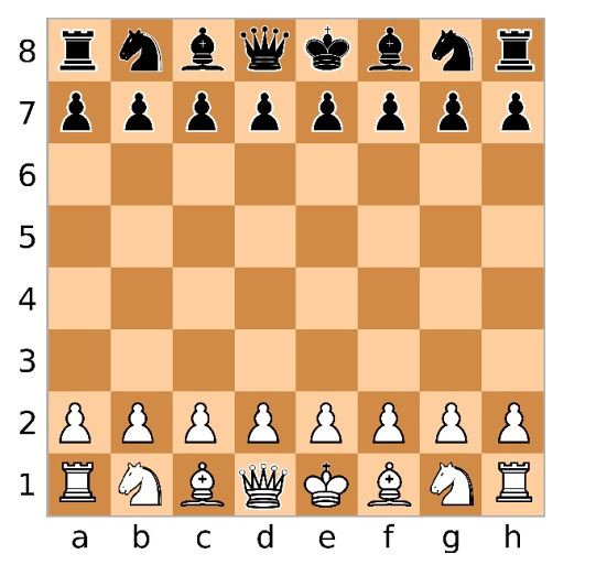
The rules of the game are as follows [PER][CHA] :
Initial setup :
Chess is played on an 8x8 checkered board, oriented with a white square in the bottom right corner.
At the start of the game, 16 white pieces and 16 black pieces are placed as follows :
- On the first rank : starting from each end, a rook, a knight, a bishop. The two central squares are occupied by the king and the queen, with the queen placed on the square of her color.
- On the second rank : the 8 pawns.
Objective
:
Players take turns.
White always moves first.
A player wins the game if they checkmate the opponent's king, or if the opponent exceeds the time limit while the player has sufficient material to checkmate them.
Movement rules :
- King : One square in any direction (horizontal, vertical, diagonal). It cannot move to a square that would put it in check.
- Queen : Any distance in any direction, provided the path is clear.
- Bishop : Any distance diagonally, provided the path is clear.
- Knight : L-shaped move (2 squares in one direction and 1 perpendicular). It is the only piece that can jump over others.
- Rook : Any distance horizontally or vertically, provided the path is clear.
- Pawn : Advances one square forward in its file (or 2 squares from its initial position, if the path is clear). It never retreats.
Capture rules :
- All pieces except the pawn capture according to their normal movement by occupying the opponent's square.
- The pawn captures only one square diagonally forward (right or left), never straight ahead.
- En passant capture : A pawn advancing two squares from its initial position and landing adjacent to an enemy pawn may be captured by that pawn on the immediately following move, as if it had only advanced one square. The capture is made diagonally onto the square the captured pawn would have occupied after a single-square move.
- The capturing piece takes the place of the captured piece, which is removed from the board.
Special rules :
- Promotion : A pawn reaching the last rank transforms into a queen, rook, bishop, or knight (choice made immediately).
- Castling : The king moves two squares in his original rank towards the adjacent rook, which then jumps over the king to its side. Two castlings are possible but only one per player per game : queenside (long) castling and kingside (short) castling. Castling conditions are :
1. Neither the king nor the relevant rook has moved previously.
2. The path between them is clear (no intervening pieces).
3. The king is not in check at the time of castling.
4. The king does not cross a checked square.
5. The king's and rook's final squares are not attacked.
- Touch-move rule : A touched piece must be played (moved if friendly, captured if enemy), unless announcing "j'adoube" (adjusting its position) before touching it.
Endgame rules :
- Check to the king : The king is under attack. Three possible defenses (PIF acronym): Capture the attacker, Interpose a piece between king and attacker, Escape the threat.
- Checkmate : The king is in check with no possible defense.
- Draw : Possible cases are :
1. Stalemate : No legal move possible, with king not in check.
2. Draw by agreement : Both players agree to end the game.
3. Triple repetition : the exact same position is repeated three times during the game, with the same player moving.
4. 50-move rule : 50 consecutive moves played by each player without capture or pawn movement.
5. Checkmate impossible due to insufficient material : Checkmate is impossible from any possible position (examples : king alone against king ; king and knight against king ; king and bishop against king ; etc.).
6. Dead position (fortress) : Checkmate is impossible from the current position (example : white king in a corner with three white pawns blocking access to the king, against black queen).
7. Time expired without possible checkmate (Article 6.9 of the FIDE for the general principle and 6.12.1 for the exception of nullity) : The game is a draw if one player exceeds the time limit and the other player has insufficient material to checkmate their opponent.
Winning Strategy :
There is no known winning strategy in Chess to date.
The optimal strategy is to minimize gross errors by following these rules [PER][CHA] :
1. Fundamental principle : Most games are won by the opponent's mistakes rather than perfect moves.
2. Develop pieces quickly :
- Bring out knights and bishops early in the opening to active squares.
- Avoid moving the same piece multiple times without necessity.
3. Ensure king safety :
- Castle early, unless there's a tactical reason not to.
- Avoid exposing the king in the center during the opening.
4. Occupy or control the center :
- Exert influence over the central squares (d4, d5, e4, e5) with pawns and pieces, either through direct occupation or remote control.
- Attack on the wings only after stabilizing the center.
- Avoid bringing out the queen too early.
5. Secure the pieces :
- Place pieces on squares where they have numerous action possibilities.
- Coordinate pieces so they support each other.
6. Structure the pawns :
- Each pawn move permanently alters the position and must be justified by a plan.
- Avoid doubled pawns (on the same file), isolated pawns (without allied pawns on adjacent files), or backward pawns (lagging on their file).
7. Exchange tactically :
- Favor piece exchanges when they improve your position.
- Simplify the position when you have a material or positional advantage.
8. Hunt threats :
- Check for threats with every move.
- Do not leave pieces hanging.
9. Exploit opponent's weaknesses :
- Doubled, isolated, or backward pawns.
- Weak squares (those no longer controlled by opponent's pawns): occupy with a knight (best choice).
- Blocked or poorly placed pieces: force unfavorable exchanges for the opponent.
- Bad bishop (bishop on squares of the same color as its pawns): never exchange it for one of your active pieces, except in rare exceptions.
10. Anticipate the endgame :
- Activate your king: it becomes an offensive piece once safe.
- Pawn structure gains increased importance.
11. Manage your time :
- Avoid consuming too much time in the opening.
B7.3. Card games :
The following card games illustrate different ways of playing with chance, where reflection, patience, and sometimes cunning influence the outcome.
B7.3.1. Prisoner Solitaire :
Prisoner Solitaire, or Accordion game, is played alone and requires a deck of 32 or 52 cards.
Rules of the game :
History tells us that it was used to pass the time for prisoners in their cells.
The rules of the game are as follows [PER][CHA] (see also the video [JEU]) :
The player holds the deck of cards face down and draws them one by one, laying them out in a single line face up on the floor or a table.
As soon as a card is framed by two adjacent cards of the same rank (any face cards or numbers, such as two 7s or two Queens) or of the exact same suit (spades, hearts, diamonds or clubs), the player places it on top of the previous card and closes the gap.
Each move back can create a new local framing and potentially a second one just before it. The player then takes absolute priority over the furthest framing that has not yet been dealt with, recursively, until no framing remains in the entire line of cards laid out.
This hierarchical rule ensures optimal handling of the framings, preventing omissions and accelerating convergence towards two final piles.
Example (see Figure above) : The cards drawn successively are as follows :
Ace of Hearts, Jack of Clubs, 8 of Spades, 5 of Hearts, Jack of Spades.
The operations are then as follows :
Ace of Hearts, Jack of Clubs, 8 of Spades, 5 of Hearts, Jack of Spades, 5 of Hearts on 8 of Spades, Jack of Clubs on Ace of Hearts, 5 of Hearts on Jack of Clubs.
The game ends here at the first layout with two single piles (5 of Hearts, Jack of Spades).
When all the cards in the deck have been drawn and all ongoing framings have been processed, the player collects the cards by stacking them from bottom to top, turns the deck face down, and begins a new layout.
The goal of the game is to reduce the layout to two single piles, which is generally achievable but very time-consuming.
However, there is a non-zero probability of failure (less than 5 % according to empirical studies). For example, during a layout, if none of the cards are framed, then subsequent layouts will reproduce the initial configuration exactly or its inverse, depending on the card-picking method.
B7.3.2. War :
War is a simple game for two players that requires a standard deck of 32 or 52 cards.
The modern rules are as follows [WIK1] :
Objective :
Cards are dealt one by one to all players, who gather them face down into a single pile.
Each player draws the top card from their pile and places it face up on the table.
The Ace is the highest card, followed by King, Queen, Jack, 10, and then descending values.
The player with the highest card wins the trick. He collects all played cards and places them under his pile.
In case of a tie - called a "war" - each player draws a new card and places it face down on top of the previous card, then a second card face up on top of those. This final card decides the winner. If another tie occurs, the process repeats as needed.
The winner is the player who collects all cards from their opponent's pile.
The game ends in a draw - even if one player clearly dominates - if a player's last card is face down or matches their opponent's value. In these cases, war cannot occur.
Variant :
There is a variant where each player receives a full deck of 32 cards at the start, shuffled independently.
The game then proceeds exactly according to the classic rules.
This variant eliminates the initial unfairness caused by splitting cards from a single deck.
However, the game length is roughly doubled.
Winning Strategy :
War is a game of pure chance with no winning strategy.
A game lasts about 30 minutes median (350 tricks) with 52 cards, or 20 minutes (250 tricks) with 32 cards - ideal for quick family play.
B7.3.3. Crapette :
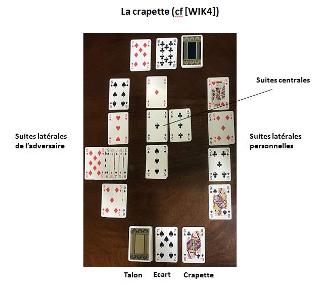
Crapette is a two-player card game belonging to the patience (solitaire) family. It requires two standard 52-card decks (without jokers).
The word "crapette" could mean "small bulging toad", by analogy with the pile of 13 hidden cards, bulging like a crouching toad, with its eye as the last visible card.
The rules below describe the flexible version of the game (often referred to as the family version) [PER][CHA].
Initial setup :
Each player uses their own deck, which they shuffle and then lay out on the table as follows (see figure above) :
- Crapette pile : Each player draws 13 cards and places them face down in a pile in front of them, to their right.
- Side sequences (or working piles) : Each player draws 4 additional cards and places them face up, to their right, forming a personal vertical column.
These cards form the beginning of the 8 side piles in play (4 personal piles and 4 belonging to the opponent).
- Central sequences : 8 central spaces, shared by both players, are left empty. They will later receive 8 card piles face up, arranged in 2 vertical columns, one for each of the 4 suits.
- Stock (talon) : The remaining 35 cards are placed face down in a pile to the left of the player's crapette pile.
- Waste pile (écart or discard) : This pile, initially empty, is located between the stock and the crapette pile. It receives, face up, cards drawn from the stock that cannot be played.
Initial tie-break :
- Each player then turns face up the top card of their crapette pile.
The player with the higher-ranked card (using the descending order : Ace, King, Queen, ..., 2) takes the first turn.
- In case of a tie, the players compare the 4 cards of their personal side sequences, position by position, from top to bottom.
Objective :
Each player must get rid of all their cards by playing them face up, according to the following possibilities :
- Central sequences :
Cards may be placed onto the central sequences, which consist of 8 ascending piles, built from Ace up to King, by exact suit (Spades, Hearts, Diamonds, Clubs).
This placement is final : once a card has been placed in a central sequence, it may not be removed.
- Side sequences :
Cards may be placed onto the side sequences, which consist of 8 descending piles, built from King down to Ace, alternating opposite colors (red/black).
This placement is temporary, as cards placed in the side sequences are intended to be transferred later to the central sequences.
- Opponent's piles :
Cards may also be placed onto the opponent's piles (crapette pile or waste pile), provided that the card played is of the same suit and of immediately higher or lower rank than the visible card of that pile (for example, a 10 of Spades on a 9 or Jack of Spades).
Players take turns. During their turn, a player may make as many plays as possible.
The winner is the first player who manages to play all of their cards onto the table.
In the event of a complete blockage of play, the player with the fewest cards remaining in total (crapette pile + waste pile + stock) is declared the winner.
Sources of draw :
A player may never draw cards from the opponent, whether from their piles or their personal side sequences.
The personal sources of draw are the following, in strict order :
- Strict order : 1. Personal crapette pile, 2. Personal stock (talon), 3. Personal waste pile
- Additional source available at any time :
The player's personal side sequences (4 piles).
Whenever a card is drawn from the crapette pile or from the stock, the next card of that pile must immediately be turned face up.
When the stock is exhausted, the player plays all possible cards from their waste pile and their crapette, then turns over the waste pile without shuffling to form a new stock.
When drawing from the side sequences, only the top card of a pile may be moved.
Placement destinations :
- Absolute priority :
The central sequences (8 piles).
- Secondary destinations :
The side sequences (8 piles, personal or belonging to the opponent) and the opponent's piles (crapette pile or waste pile).
Cards are always played or moved one at a time.
All cards in the side sequences must be visible, with the card played not completely covering the previous one.
The side sequences may only be reorganized through successive moves of cards taken from the tops of the piles. An empty space in a side sequence may receive any card.
Fouls :
A foul occurs whenever a player violates any of the rules stated above, in particular :
- Failing to place, as a priority, a card from one of their piles (crapette, stock, waste) onto the central sequences.
- Drawing a card from the stock while a card from the crapette pile could be played.
- Drawing a card from the waste pile while a card from the stock or from the crapette pile could be played.
Whenever a foul is committed, the opponent calls "Crapette !".
The player at fault leaves the rest of the layout unchanged, then places the incorrectly played card onto their waste pile, then immediately ends their turn, which passes to the opponent.
Common variants :
1. No drawing order variant :
The drawing order (crapette pile, stock, waste pile) is removed. The player may freely draw from any of these piles. This variant favors fluidity and optimization of sequences over the traditional priority constraint, turning crapette into a freer and more tactical game.
2. Variant with shared side sequences : The side piles are shared and not assigned to individual players, therefore without the personal/opponent distinction. The side piles can be manipulated by both players. This variant greatly increases the tactical depth and the potential for rearranging the piles.
Winning Strategy :
There is no winning strategy for Crapette. However, there exists a set of guiding principles to implement according to the following hierarchical order [PER][CHA] :
1. Play on the central piles to avoid a fault and advance the central game.
2. Create a maximum of empty spaces in the side sequences by two possible means : restructure the side sequences (often to merge several short ones into a single long one), and load the opponent's two piles.
3. Free the crapette pile by accompanying, when possible, the crapette card with the one from the stock or the waste pile, unless this freeing gives the opponent a favorable restructuring.
Each game takes about 20 minutes.
B7.3.4. Poker :
Poker is a strategic card game played by 2 to 10 players, using a standard 52-card deck.
Its main goal is to win the bets (the "pot"), either by forming the best five-card combination or by forcing opponents to fold through bluffing.
The four most played poker variants worldwide are Texas Hold'em, Omaha, 7-Card Stud, and 5-Card Draw.
A game refers to the set of hands played at a table, while a hand corresponds to one complete deal, from the initial bet to the pot award.
Warning : in English, the word "hand" can refer either to a hand of cards (combination) or to a round of play (deal).
Types and Values of Cards :
Two types of cards are possible :
- private cards, unique to each player, which can be hidden, called "closed" (visible only to that player) or visible, called "open" (revealed to the other players),
- community cards, visible and usable by all players.
According to the variant, the dealt cards are distributed as follows :
- Texas Hold'em : 2 hidden private cards and 5 community cards.
- Omaha : 4 hidden private cards and 5 community cards.
- 7-Card Stud : 3 hidden private cards and 4 visible private cards.
- 5-Card Draw : 5 hidden private cards, revealed only at showdown.
The card values are as follows, ranked in increasing order of strength :
2, 3, 4, ..., 10, Jack (J), Queen (Q), King (K), Ace (A), with the Ace also able to count as 1 in allowed straights (e.g., A-2-3-4-5).
In 4- or 5-player games, it is common to remove the 2, 3, and 4, reducing the deck to 40 cards.
Hand Hierarchy [WIK9] :
The hierarchy of hand strengths is as follows, with their probability of occurrence for a 52-card deck in two cases :
- List 1 : random 5-card draw, typical of the 5-Card Draw variant.
- List 2 : best hand from 7 cards, for Texas Hold'em, Omaha, and 7-Card Stud variants.
This hierarchy remains the same across all poker variants. Only their probabilities of occurrence vary, depending on the number of cards dealt and those that can be combined to form the best hand.
Each hand is defined by its minimal criterion, with the hand hierarchy automatically resolving overlapping cases.
| Hand | Definition | Example | Tiebreaker | Probability List 1 | Probability List 2 |
|---|---|---|---|---|---|
| Royal Flush | Straight flush with Ace-high | 10 J Q K A | impossible | 0.00015 % | 0.0032 % |
| Straight Flush | 5 consecutive values, same suit (Ace low allowed) | 8 9 10 J Q | highest card | 0.0014 % | 0.028 % |
| 4-of-a-Kind | 4 cards of same value | Q Q Q Q | value of 4-of-a-Kind, then kicker | 0.024 % | 0.17 % |
| Full House | 3-of-a-kind + pair | 10 10 10 K K | three value, then pair | 0.14 % | 2.60 % |
| Flush | 5 cards same suit | 8 9 10 J K | cards descending | 0.20 % | 3.03 % |
| Straight | 5 consecutive values (Ace low allowed) | 8 9 10 J Q | highest card | 0.39 % | 4.6 % |
| 3-of-a-Kind | 3 cards same value | 10 10 10 | value of 3-of-a-Kind, then kickers descending | 2.11 % | 4.83 % |
| Two Pair | Two pairs | K K 8 8 | highest pair, second pair, kicker | 4.75 % | 23.50 % |
| One Pair | 2 cards same value | K K | pair value, then kickers descending | 42.26 % | 43.82 % |
| High Card | None of above | A J 9 6 2 | cards descending | 50.12 % | 17.41 % |
| Total | 100,00 % | 100,00 % |
Note in this table :
- Suit color does not affect a hand's intrinsic strength in the hierarchy relative to other hands, except to form a Flush, Straight Flush, or Royal Flush. Among themselves, suits are equivalent and neutral, except to break ties in some non-standard variants.
- Probabilities do not always increase strictly with hand weakness, but the hierarchical order remains correct for determining the winner.
Entry fee (bankroll) :
The bankroll is the amount each player stakes to participate in the game.
- At the start of the game, the player buys chips corresponding to their bankroll.
- During the game, all bets and raises are made solely with chips.
- At the end, the player exchanges their chips for money according to their value.
Bet before card dealing (initial bet) :
Before any card dealing, a mandatory bet is required to form the starting pot.
It takes the form of antes (all players bet) or blinds (forced bets by certain players), made without knowledge of the cards.
Ante :
The ante is an identical mandatory bet placed by each player before the cards are dealt to create an initial pot.
It is mandatory in the 7-Card Stud variant and optional in 5-Card Draw.
Blind :
The blinds are forced bets placed before the cards are dealt to create an initial pot.
They are mandatory in Texas Hold'em and Omaha variants, and may be combined with antes depending on the game's specifics.
Two types of blinds exist :
- Small Blind (SB) : small bet, placed by the player immediately to the left of the dealer button.
- Big Blind (BB) : full bet (typically double the SB), placed by the player to the left of the Small Blind.
The other players, excluding SB and BB, do not bet initially.
The straddle (or sur-blind) is an optional additional bet (typically double the BB), placed by the player to the left of the Big Blind.
It provides a strategic advantage by allowing the straddler to act late on the first betting round, increasing the initial pot and putting pressure on opponents.
Card dealing (the deal) :
Cards are dealt one by one, clockwise, starting from the player to the dealer's left, according to the variant played.
The dealer's role rotates each hand.
Game flow :
After the deal, players bet through successive betting rounds, according to the variant's stages.
Action consists of making a decision : fold, call, or raise.
It starts with the player to the left of the blinds during betting rounds and proceeds clockwise.
Without blinds, action starts with the player to the left of the dealer (5-Card Draw) or the player with the lowest visible card (7-Card Stud).
The basic principle of betting is that a player must "call" by matching the highest bet to stay in the hand. If they don't, they "fold" and lose their bets already committed. They can also"raise", i.e. increase the bet, forcing other players to call, raise, or fold.
A betting round ends when all remaining players have either folded or matched the highest bet.
Betting rounds :
A hand consists of several betting rounds depending on the variant.
For each round, the number of cards indicated below is the number of cards dealt, revealed, added, or exchanged, made available to the player, whether they are private or community cards.
Texas Hold'em and Omaha : 4 rounds
- Preflop : 2 private cards for Texas Hold'em and 4 for Omaha
- Flop : 3 community cards
- Turn : fourth community card
- River : fifth and final community card
7-Card Stud : 5 rounds
- 3rd Street : 3 cards (2 hidden, 1 visible)
- 4th Street : 1 visible card
- 5th Street : 1 visible card
- 6th Street : 1 visible card
- 7th Street : 1 hidden card
5-Card Draw : 2 rounds
- After the deal : 5 cards
- After the draw : 0 to 5 cards
Card Exchange :
Depending on the variant, a player may or may not exchange cards, which are drawn from the deck by the dealer or by the professional dealer in a casino.
In Draw-type variants (especially 5-Card Draw), card exchange is allowed after the first betting round.
In other common variants (Texas Hold'em, Omaha, 7-Card Stud), no exchange is possible : cards are only dealt during the deal.
End of hand :
The hand ends either by all players but one folding (winner takes the pot), or by showdown after the final betting round.
Winning strategy :
There is no winning strategy in poker, but there exists an optimal beginner strategy that consists of following these principles [PER][CHA] :
1. Play for expectation : A decision is good if it is profitable in the long term, even if it sometimes leads to an immediate loss.
2. Adapt your strategy to your position : Play cautiously when acting early in the betting rounds, and aggressively by exploiting available information when acting late, ideally last.
3. Adapt your bets to the situation : Bet big when you have good cards or to protect the pot, and bet small or fold otherwise.
4. Bluff intelligently : Bluff just enough to make the opponent indifferent between calling and folding.
5. Play the opponents : Bluff more against cautious players and less against calling players.
6. Manage your stack : Never risk too much on a single hand and know when to leave the table.
7. Play tight : For a deliberately cautious strategy, participate in only about 20 % of the hands in a game, hence the ultra-simple rule depending on the variant :
- 5-Card Draw : Fold unless you have a high pair (JJ, QQ, KK, or AA), or better, from the deal.
- Texas Hold'em : Fold unless you have a pair, an Ace with a high card, or two consecutive cards of the same suit (suited connectors), preflop.
- Omaha : Fold unless you have two possible Flush hands with suited cards (double suited draw), or a strong pair (AA or KK), preflop.
- 7-Card Stud : Fold unless you have a hidden high pair or three cards that can form a Straight or Flush, after the third card.
B7.4. Dice games :
The following dice games are games that combine chance and strategy.
B7.4.1. Pig :
Pig, also known as 101 Game, is a simple dice game for two or more players that combines chance and strategy.
Be careful not to confuse it with "Le Cochon qui rit" (assembling a miniature or drawn pig) or "Pass the Pigs" (pig-shaped figurines used as dice).
The game relies on a balance between risk-taking and caution, with each player choosing the right moment to stop before rolling a 1 wipes out everything.
The game requires a standard six-sided die, a sheet of paper and a pencil to track scores.
The rules of the usual game are as follows [WIK6] :
Initial setup :
Each player's total score starts at 0.
Objective :
Players take turns.
On their turn, a player rolls the die as many times as they wish.
As long as the result is not 1, they add the value obtained to their turn points.
They can then choose to roll again to try to gain more or stop to secure the turn points and add them to their total score.
However, if they roll a 1, all turn points are lost (but not the total score points), and their turn ends immediately.
The winning player is the one who reaches or exceeds 101 points on their total score at the end of their turn.
Variant :
A harsher variant consists of resetting the player's total score to 0 when they roll a 1.
Winning Strategy :
There is no winning strategy for Pig because chance dominates. However, there exists an optimal strategy based on mathematical probability analysis, according to the following rules [PER][CHA] :
1. The optimal number of points to aim for per turn is around 20 points (optimal threshold to maximize expected gain).
2. This threshold should be decreased as the total score approaches 101 to reduce risk against the opponent : typically 15 points from a total score of 70 points, then 10 points from 91 points.
These thresholds come from mathematical analysis per isolated turn : Each additional roll has a positive expected gain, but also a 1/6 risk of losing all turn points. This expectation becomes unfavorable when accumulated turn points approach 20.
Demonstration :
The average value of a roll, conditional on not rolling 1, is : (2 + 3 + 4 + 5 + 6)/5 = 4
The probability of not rolling 1 is : 5/6
The raw expected value of an additional roll is therefore : (5/6) 4
But the risk of losing accumulated turn points must be considered. If the player already has T points in the turn, the net expected value E(T) of rolling again is : E(T) = (5/6) 4 - (1/6) T = 3.33 - T/6
Rolling again therefore remains favorable as long as : T < 20
B7.4.2. Yahtzee :
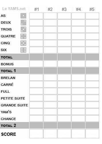
Yahtzee is a dice game for one or more players that combines chance and strategy.
Each player aims to form dice combinations to maximize their score on a dedicated scoresheet.
The game originated in Canada in the 1950s under the name "Yacht Game". It was created by a couple who introduced it to their guests during yacht cruises. The game was then popularized and marketed in 1956 as Yahtzee by Edwin S. Lowe.
The game requires 5 standard six-sided dice, a sheet of paper and a pensil for scoring.
The rules for the standard (family) game are as follows [PER][CHA] :
Initial setup :
The scoresheet has as many columns as players and as many rows as possible combinations (see Figure above).
Rows are divided into two sections :
- Upper Section : Each row corresponds to a dice value (Aces, Twos, ..., Sixes).
Aces : Sum of dice showing 1s. Score = this sum (example : 1-1-1-1-6 = 4 points).
Twos : Sum of dice showing 2s. Score = this sum.
Threes : Sum of dice showing 3s. Score = this sum.
Fours : Sum of dice showing 4s. Score = this sum.
Fives : Sum of dice showing 5s. Score = this sum.
Sixes : Sum of dice showing 6s. Score = this sum.
Total : Sum of the six scores above.
Bonus : +35 points if Total ≥ 63 points.
Total 1 : Total + Bonus
- Lower Section :
3-of-a-Kind : At least 3 identical dice. Score = sum of those dice (example : 2-2-2 = 6 points).
4-of-a-Kind : At least 4 identical dice. Score = sum of those dice (example : 3-3-3-3 = 12 points).
Full House : A triplet and a pair of identical dice (example: 3-3-3-6-6). Score = 25 points.
Small Straight : At least 4 consecutive dice (example: 2-3-4-5). Score = 30 points.
Large Straight : At least 5 consecutive dice (example: 2-3-4-5-6). Score = 40 points.
Yahtzee : 5 identical dice (example : 4-4-4-4-4). Score = 50 points.
Chance : Any combination. Score = total of all five dice. This saves a turn by avoiding crossing out a combination.
Total 2 : Sum of the seven scores above.
Final score : Total 1 + Total 2
Objective :
Players take turns.
On their turn, the player rolls the five dice, not exceeding three rolls total (initial roll plus two optional re-rolls).
After each roll, they may keep all or some dice as they wish to try to form the desired combination.
At the end of their turn, they must fill one empty box on the scoresheet.
If no combination is possible or worthwhile, they must cross out a combination of their choice.
The game ends after 13 turns corresponding to the 13 combinations, when all boxes on all players' sheets are filled.
The winner is the player with the highest score in the Final score row.
Variant - Upper Section line blocking :
When a player achieves the maximum possible score in an Upper Section row, that row becomes inaccessible to all other players for the rest of the game.
For example, a player rolls 3-3-3-3-3 in the Threes row. The Threes row is then crossed out for all other players.
Winning strategy :
There is no guaranteed winning strategy for Yahtzee because chance dominates. However, an optimal strategy exists based on these principles [PER][CHA] :
1. Upper Section : Aim for the 35-point Bonus and blocking Upper Section lines.
2. Variable scores (Upper Section, 3-of-a-Kind, 4-of-a-Kind) : Always re-roll up to the 3rd roll to maximize the score.
3. Fixed scores (Full House, Small Straight, Large Straight) : Stop immediately once the combination is obtained.
4. Chance : Reserve for high dice totals, or as a last resort to avoid crossing out a combination.
5. Overall strategy (timing) :
- Early game (turns 1-4) : Prioritize fixed scores (Full House, Small/Large Straight) which are relatively accessible and free up the Upper Section for later.
- Mid-game (turns 5-9) : Target variable scores (Upper Section, 3/4-of-a-Kind) to accumulate high points, including the Bonus.
- Late game (turns 10-13) : Aim for Yahtzee and Chance with high dice totals to maximize the Final score or save remaining empty boxes.
B7.5. Games on paper :
The following games, easy to set up with just a sheet of paper and a pencil, involve strategies based on controlling the game space.
B7.5.1. Battleship :
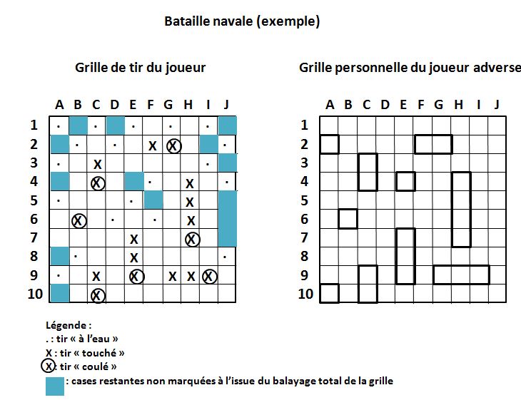
Battleship, also known as Touché-Coulé, is a two-player board game where opponents secretly place "ships" on a grid and try to "hit" each other's ships.
Standard French/Belgian rules are as follows [WIK2] :
Initial setup :
Each player uses two 10x10 numbered grids (French style : rows 1-10 top to bottom, columns A-J left to right).
Each player commands a fleet of 10 ships represented by rectangles 1-4 squares long :
- 1 large ship (4 squares)
- 2 medium ships (3 squares each)
- 3 medium ships (2 squares each)
- 4 small ships (1 square each)
L-shaped, T-shaped, square, zigzag or discontinuous shapes are forbidden.
The personal grid shows your own fleet. At game start, place all ships vertically or horizontally, drawing each as a bold rectangle.
Ships must be separated by at least one empty square (no corner touching). Empty squares represent water.
The firing grid tracks the opponent's territory, where you will hunt their ships.
Objective :
Players take turns calling out a grid square (e.g., "B6"). The opponent must respond with one of these announcements :
- "Miss" if the shot lands in water
- "Hit" if the shot strikes a ship but leaves intact squares
- "Sunk" if the shot hits the last intact square of a ship.
On their firing grid, the player marks :
- A dot (.) for a "miss"
- An X for a "hit"
- A circled X (⊕) for a "sunk". Immediately after this shot, the player must also mark with a dot (.) all unmarked squares surrounding the sunken ship in order to materialize the non-contact rule.
The winner is the first player to "sink" all of the opponent's ships.
Example :
The Figure above shows an example of Battleship, with the opponent's personal grid (unknown to the player) and the player's firing grid.
The first shot is fired at square A1. Subsequent shots are fired row by row, from left to right and top to bottom, according to the optimal strategy (see below).
To avoid cluttering the Figure, the firing grid does not include the additional markings (.) placed on unmarked squares surrounding sunken ships immediately after a "sunk" shot.
After this firing grid has been completely scanned, all ships of size 2 squares or more are sunk. Only 3 small ships of size 1 square (A2, E4, and A10) remain to be found in a maximum of 14 shots (shaded squares in the Figure).
Variant :
Each player fires a volley of three shots in succession. This variant speeds up the game.
Winning Strategy :
No winning strategy is known for Battleship. However, an optimal strategy exists based on these rules [PER][CHA] :
1. Placement phase : Maximum dispersion.
- Distribute the ships across the entire grid to limit spatial correlations and make any local information less useful.
- Prioritize the center of the grid. Central squares allow for more possible placements, enabling ships to blend into the surrounding uncertainty (statistical camouflage).
- Avoid corners and clusters. In intuitive exploration, these areas are subject to psychological targeting ("suspicious zones"). In systematic exploration (checkerboard pattern), corners are hit by early shots, and clusters encourage concentrated shots that can trigger the abandonment of the systematic search in favor of a targeted search.
2. Search Phase : Minimum number of shots.
- Mentally color the opponent's grid according to a checkerboard pattern with alternating black and white squares (like on the checkers board of International Draughts).
- Choose a color and then systematically scan the squares of that color. Only fire at squares not already marked with (.), (X), or (⊕).
- As soon as a shot is called as "hit," abandon the search and proceed to the pursuit phase.
- This scan with a maximum of 50 shots will sink all ships of size 2 squares or more.
- After this scan, search for the remaining ships of size 1 square by randomly shooting at the n remaining unmarked squares (n = 15 on average). The average number of shots (E) to find the k remaining ships is then 12 shots if k = 3 (according to the formula E = k (n + 1)/(k + 1)).
3. Pursuit phase (after a "hit") : Tenacity.
- Immediately target orthogonal adjacent squares to locate and destroy the hit ship.
- Determine ship orientation (vertical or horizontal) after the second hit.
- Continue in the corresponding direction until complete destruction of the ship.
- Never return to global search until the ship is sunk.
B7.5.2. Racetrack :
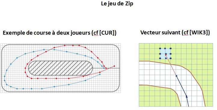
The Zip game, also known as Formula 1, Paper Race, or Racetrack - popularized by Martin Gardner in 1973 - is a fun game where one or more players compete in a speed race on a track drawn on graph paper, realistically incorporating acceleration and braking constraints.
The basic rules are as follows [WIK3] :
Initial setup :
The game requires graph paper (preferably large squares), an eraser, and one pencil per player (preferably in different colors).
The track is drawn on the paper with two more or less parallel winding boundaries, ending in a straight start line as wide as the number of players in squares, and a finish line.
Track boundaries can only be straight line segments to avoid disputes.
The track can also be a closed loop with the same start and finish line (see figure above).
Each player marks their car's starting position with a pencil on one of the grid points on the start line.
Objective :
Players then take turns.
The winner is the first player to touch or cross the finish line.
Movement rules :
1. Any move landing on a position already occupied by another player is forbidden.
2. The first move is one square forward along the track, represented by a vector from the starting point to one of its three neighboring points in the direction of the race.
3. On each turn, the player extends the previous move by plotting that vector from their current position. The resulting point is called the principal point. The player may also choose to move to one of the eight neighboring points of the principal point (see Figure above). These choices simulate the maximum acceleration or braking allowed given the car's inertia.
Fouls :
1. When a player leaves the track by crossing one of its boundaries, one of the following two types of penalties is applied on the next turn (to be agreed upon before the game starts) :
- Soft penalty (emergency braking) :
The player skips their turn. On the following turn, the vector corresponding to the off-track exit is reset to zero. The player restarts by moving to one of the eight neighboring points of their position (the principal point coincides with the current position).
This rule penalizes the mistake without eliminating the player from the race, giving them a second chance to win.
- Strict penalty (recovery race) :
The player must re-enter the track by crossing the boundary at a point located behind the point where they left the track. The higher the speed at the moment of exit, the greater the number of moves required to return to the track.
This rule significantly reduces the chances of winning after a mistake.
2. On some very twisty tracks, it may happen that a move off the track corresponds to a vector that crosses the track boundary twice, with both the starting point and the ending point lying inside the track. This kind of "risky shortcut" is allowed and does not count as going off the track.
Winning Strategy :
There is no winning strategy in the Zip game. However, an optimal strategy exists based on the following rules [PER][CHA] :
1. Anticipate turns by slowing down progressively to maximize average speed over the entire race.
2. Avoid sudden accelerations and sharp direction changes to reduce the risk of going off-track.
3. In turns, negotiate curves like a race car driver : approach the turn hugging the outer edge of the track. During the turn, maintain this trajectory as long as the turn's exit is not visible. Then, progressively cut the corner to rejoin the straight line. This trajectory minimizes the distance traveled within the curve and helps preserve a high exit speed.
B7.5.3. Gomoku-style game on 10 10 grid :
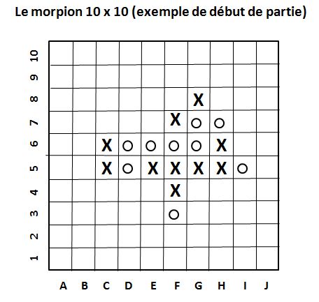
Gomoku-style game on 10 10 grid, or "Extended Tic-Tac-Toe", is a strategic two-player game where the goal is to be the first to align a series of 5 identical symbols on a 10x10 grid.
The basic game rules are as follows [WIK7] :
Initial setup :
The game requires a squared grid paper (typically 10 x 10) and a pencil per player.
The grid is empty at the start of the game.
Each player chooses a distinct symbol : X or O
Player X always starts and therefore has an advantage, not geographical (position on the grid), but functional (offensive role with always one move ahead).
To restore balance, the "pie rule" can be applied. After X's first move, player O chooses either to keep their O role or to swap symbols (they become X and their opponent becomes O). Depending on the quality of the first move or their personal preference, player O can thus freely choose their role (offensive or defensive) for the rest of the game, each role offering interest according to the player's playing style.
Objective :
Players take turns.
On their turn, a player places one symbol in an empty square. The symbol is permanent and cannot be removed or moved.
The winner is the first player to create an alignment of at least 5 identical consecutive symbols, horizontally, vertically, or diagonally (See example of the game start in the Figure above).
If the grid is completely filled without any alignment formed, the game is declared a draw.
Variant :
The game ends when the grid is completely filled. The winner is the player with the most winning alignments.
A winning alignment is a series of at least 5 identical symbols in a row without a break (streaks of 6 or more (overlines) also count as winning alignments). Short or long series count as a single alignment and cannot overlap or intersect.
Winning strategy :
There is no guaranteed winning strategy in Gomoku-style game on 10 10 grid. However, there exists an optimal strategy based on the following rules [PER][CHA] :
Rules to prioritize in the following order (Legend : 'X' for the player, 'O' for the opponent, '_' for an empty square) :
1. Immediate victory : Complete an XXXX_ or XXX_X or XX_XX or X_XXX
2. Defeat avoided : Absolutely block an OOOO_ or OOO_O or OO_OO or O_OOO
3. Fork avoided : Absolutely block an opponent's potential fork.
4. Double attack (fork) : Place an X creating two immediate threats simultaneously in two distinct lines, each forming an alignment of four X's with one empty square either at the end or within the alignment.
5. Simple attack : Create an XXXX_ or XXX_X or XX_XX or X_XXX
6. Extend alignments : Always extend existing alignments (rather than playing isolated).
7. Center + intersections : Prioritize the grid center and intersection squares (empty squares at the crossroads of two or more existing alignments).
B7.5.4. Tic-tac-toe :
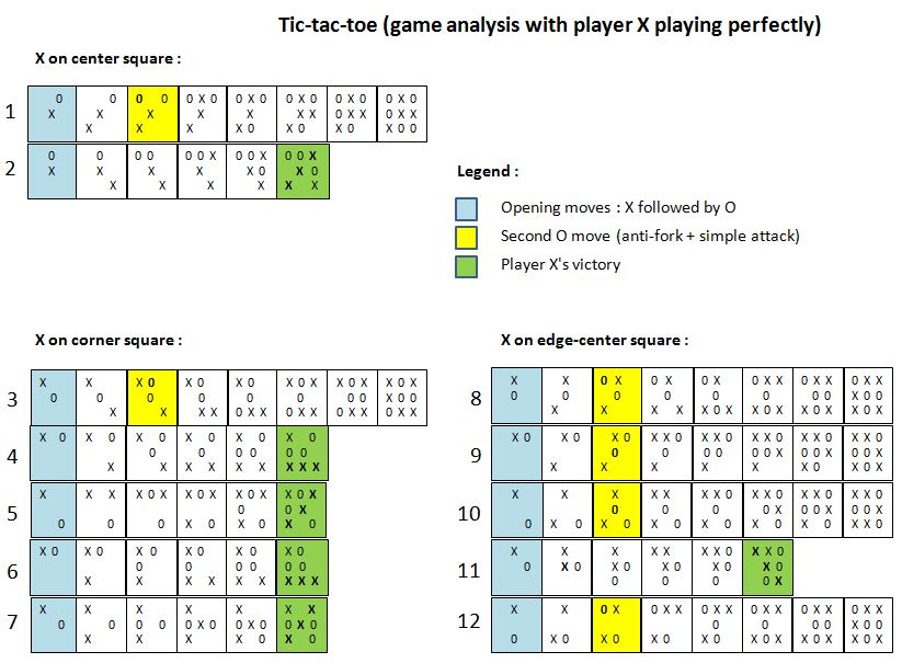
Tic-tac-toe is the standard reduced version of Gomoku-style game on 10 10 grid [WIK8]. The differences with the 10 10 version are as follows :
- 3 3 grid (instead of 10 10) with reduced square notation (A1, A2, A3, B1, B2, B3, C1, C2, C3).
- Alignment of 3 identical symbols (instead of at least 5 consecutive identical symbols).
- Possible replacement of the "pie rule" balance rule by the rule where each player plays two games, one as X and one as O. The winner is the player who wins at least one of the two games without losing any. In all other cases, the match is declared a draw.
- Victory on first alignment (the variant counting multiple alignments is excluded).
- Specific optimal strategy due to the immediate presence of grid edges (see below).
Game analysis :
If both players play perfectly, the game always ends in a draw.
Player X starts the game. Their first move can belong to one of three distinct position classes on the board : the central square, one of the corners, or one of the edge-center squares.
Player O responds with a move that can belong to one of five distinct position classes : the central square, one of the corners (adjacent or distant from X's square), or one of the edge-center squares (adjacent or distant from X's square).
This leaves 12 possible cases excluding equivalent cases by symmetry (see Figure above), with the following outcomes when player X plays perfectly :
- If X plays the central square, the game is won by X if O mistakenly plays an edge-center square (case 2 of the Figure), and drawn otherwise (O plays a corner square).
- If X plays a corner square, the game is won by X if O mistakenly plays a corner square or edge-center square (cases 4 to 7 of the Figure), and drawn otherwise (O plays the central square).
- If X plays an edge-center square, the game is won by X if O mistakenly plays an edge-center square adjacent to X's (case 11 of the Figure), and drawn otherwise (O plays the central square, a corner square, or the edge-center square opposite to X's).
The optimal opening strategies for each player are then as follows :
*
Player X :
-
To avoid unfavorable cases - in particular case 11 (X on an edge-center square followed by O on an edge-center square adjacent to X) - player X must open either on the center square or on one of the corners (cases 1 to 7).
-
In the majority of O's possible replies (cases 2, 4, 5, 6 and 7), this opening places X in a practically winning position.
- In the remaining cases (cases 1 and 3), X leaves O with a delicate defensive situation as early as O's second move, where O must play a often unique move combining fork prevention and a simple attacking threat in order to maintain a draw.
-
Any victory by player X therefore relies on a mistake by player O.
*
Player O :
- On O's first move, O must play the center square if it is free otherwise, one of the corners adjacent to X's initial square (cases 1, 3, 8, 9), immediately eliminating certain unfavorable cases. This strategy guarantees a draw if both players play perfectly. Any other response may lead to a defeat for O.
-
On O's second move, O must imperatively play the (often unique) square that simultaneously neutralizes all potential forks by X and forces X to respond to an O alignment, whenever such forcing is possible (see the squares highlighted in yellow in the Figure).
-
Player O is thus doubly disadvantaged : to secure a draw, O must play without any error in the two critical opening moves : the first (center or adjacent corner) and the second (anti-fork + simple attack).
-
Any victory by player O therefore requires a mistake by player X.
Winning strategy :
There is no guaranteed winning strategy in Tic-tac-toe. However, there exists an optimal strategy based on the following rules [PER][CHA] :
Rules to prioritize in the following order (Legend : 'X' for the player, 'O' for the opponent, '_' for an empty square) :
1. Immediate victory : Complete an XX_ or an X_X
2. Defeat avoided : Absolutely block an OO_ or an O_O
3. Fork avoided : Absolutely block an opponent's potential fork.
4. Double attack (fork) : Place an X creating two immediate threats simultaneously in two distinct lines, each forming an alignment XX_ or X_X
5. Simple attack : Create an XX_ or X_X
B7.6. Lottery games :
Lottery games, such as Loto, roulette, or slot machines, form a vast family of gambling games where chance prevails over strategy. In the long term, the player incurs inevitable losses due to a negative mathematical expectation.
In approximate percentage of the participation cost, the player's average loss per unit of bet (one grid or one token) is indeed as follows :
- French Lotto FDJ (60 %)
- EuroMillions (50 %)
- Rapido (33 %)
- Scratch-off ticket (45 %)
- Boule (11 %)
- American Roulette - special 5-number bet (8 %)
- Classic 3-reel slot machine (6 %)
- American Roulette - other bets (5 %)
- French Roulette (3 to 1 % depending on special rules)
We thus observe that lotteries like Loto redistribute little to players, while better-structured casinos lead to lower losses, especially on French roulette.
Warning : Gambling organizations often announce a global redistribution rate (RTP) calculated from winnings weighted by their probability.
This rate is doubly misleading : rounded upward and, above all, masking the player's real loss. For example, in the game of Boule, the advertised RTP of 90 % actually corresponds to a negative expected value per bet (E = TRG - 1) of -11 %
B7.6.1. French Lotto :
The French Lotto is an individual or collective game of chance, with very limited strategic dimensions.
Two main variants exist :
- Traditional Lottery : Practiced during local festivals or in an associative setting, with game cards featuring 90 numbers.
- FDJ Televised Lottery : Offered by La Fran aise des Jeux (FDJ), with grids of 49 numbers + 10 numbers for the Chance number.
B7.6.1.1. Traditional lottery [PER][CHA] :
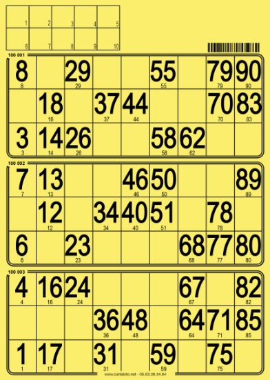
Materials :
- Drawing machine : Bingo cage or equivalent device.
- Balls : 90 balls numbered from 1 to 90.
- Game cards : Predefined cards distributed to players before the game (see Figure above).
- Each card contains 1 to 3 grids.
- Each grid = 3 rows 9 columns.
- Each row = 5 numbers and 4 empty spaces.
- Some cards have 2 rows of 5 numbered boxes (1 to 10) in the top left corner for administrative reference.
- All cards and all grids participate in the same draw, but winnings are calculated per grid.
Grid Filling :
- Players mark the drawn numbers on their grids.
- Empty spaces must not be marked. Any stray mark results in grid invalidation.
- Each grid is independent. Using multiple grids simply multiplies winning chances.
Winning Conditions :
- A win occurs when one of the following figures is obtained on a grid :
-
Quine : 5 marked numbers on a horizontal line.
-
Double quine : 10 marked numbers on two horizontal lines.
-
Full grid : 15 marked numbers across the entire grid.
- Only horizontal lines count. No other configuration (vertical, diagonal) is valid.
- Winnings amounts per grid are given in the following table :
| Figure | Gain (G) | probability (p) |
|---|---|---|
| Quine | Defined by organizer | 1/43 949 268 |
| Double quine | Defined by organizer | 1/(5,72 1012) |
| Full grid | Defined by organizer | 1/(4,58 1016) |
Note on this table :
The probability (p) represents the theoretical minimum probability, corresponding to a figure obtained exactly at the earliest possible moment.
In practice, the draw continues, which slightly increases the probabilities. Additionally, playing multiple grids increases the probabilities proportionally to the number of grids played.
The probability (p) is calculated as follows, with n = number of winning numbers required (5, 10, or 15) :
p(n) = C(n, n) C(90 - n, 0) / C(90, n) = 1/C(90, n) with :
Binomial coefficient C(a, b) = a! / (b! (a - b)!)
C(n, n) = 1 : number of ways to choose n winning numbers among the n numbers forming the figure.
C(90 - n, 0) = 1 : number of ways to choose zero losing numbers among the (90 - n) remaining numbers.
C(90, n)
: total number of possible draws of n numbers from 90.
The probabilities associated with the different figures (quine, double quine, and full grid) are therefore extremely low, practically negligible.
Draw procedure :
- Draw dates are set by the lottery organizer.
- Each figure (quine, double quine, full grid) is associated with a maximum number of balls that can be drawn, typically : 40 for the quine, then 20 additional for the double quine and 15 additional for the full grid. These cumulative limits are announced at the start of the evening by the organizer.
- The draw begins after card distribution.
- Numbers are drawn one by one, then announced or displayed.
- A player believing they have a figure raises their hand and announces it clearly.
- The draw is interrupted to verify and validate winnings.
- It continues until all planned figures are achieved or until all 90 numbers are exhausted.
Winning stratégy :
There is no winning strategy for traditional lottery. Unlike the FDJ Lottery where rational risk management remains possible, traditional lottery offers no viable strategy : neither grid choice (fixed card imposed), nor control over draws (sequential without intervention).
Given the extremely low probabilities associated with the different figures, traditional lottery cannot be considered a game of gain, but solely as a collective entertainment game.
B7.6.1.2. FDJ Televised Lottery [PER][CHA] :
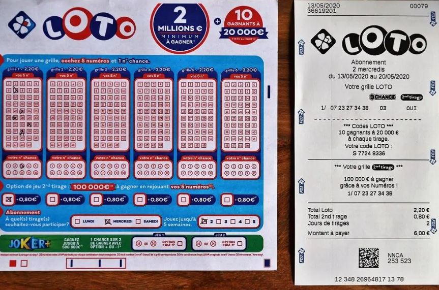
Materials :
- FDJ drawing machine.
- Balls : 49 balls numbered from 1 to 49 for the 5 main numbers. A complementary ball ("Chance number") is then drawn from 10 balls numbered from 1 to 10.
- Game slips : purchased at tobacco shops (see Figure above).
- Each slip contains 1 to several grids to be freely filled by the player or automatically proposed by the FDJ terminal (Flash mode).
- Each grid = 5 numbers chosen from 49, and 1 optional number ("Chance number") chosen from 10.
- FDJ terminal in tobacco shops, featuring two input options (manual/Flash), a bulletin scanner, and paper output (participation receipt and legal proof).
Grid filling :
- Players fill their grids before the draw.
- Each grid is independent. Using multiple grids simply multiplies winning chances.
Winning conditions :
- A win occurs on a grid based on the number of correct numbers, including the complementary number.
- Winnings amounts for a single grid are given in the following table :
| Combinaison | Gain (G) | probability (p) |
|---|---|---|
| 5 + Chance | Jackpot (2 000 000) | 1/19 068 840 |
| 5 | 200 000 | 1/1 906 884 |
| 4 + Chance | 800 | 1/86 676,55 |
| 4 | 300 | 1/8 667,655 |
| 3 + Chance | 40 | 1/2 015,73 |
| 3 | 20 | 1/201,573 |
| 2 + Chance | 7 | 1/143,98 |
| 2 | 4 | 1/14,398 |
| 1 + Chance | 2,20 | 1/28,09 |
| 1 | 0 | 1/2,809 |
| 0 + Chance | 2,20 | 1/17,56 |
| 0 | 0 | 1/1,756 |
Note on this table :
1. The gain (G) represents the gain (G) in euros, paid by the FDJ per standard grid for a participation cost c = 2.20 euros, corresponding to FDJ's official payout scale, which varies by draw. The G values shown are illustrative but plausible examples.
2. The probability (p) is the probability that a given combination results in gain G. It is calculated as follows, with n = number of winning numbers :
p(n) = C(5, n) C(44, 5 - n) / C(49, 5) and p(n + Chance) = p(n) x 1/10 with :
Binomial coefficient C(a, b) = a! / (b! (a - b)!)
C(5, n) : number of ways to choose n winning numbers among the 5 drawn.
C(44, 5 - n) : number of ways to choose (5 - n) losing numbers among the 44 not drawn.
C(49, 5)
: total number of possible combinations of 5 numbers among 49
3. The mathematical expectation (E) of the grid is the difference between the expected gain ∑i [Gi pi] and the cost c, i.e.: Egrille = -1,297 euros
On average, for each single grid, the player therefore loses approximately 1.30 euros on a 2.20 euros cost, i.e. nearly 60 % of the amount wagered.
Draw procedure :
- Official draw dates are: Monday, Wednesday, and Saturday evenings.
- The draw is broadcast live or on official platforms.
- The 5 main numbers and the complementary number are drawn continuously.
- Results are individually verified after the draw.
- Winnings are automatically awarded according to official rules.
Winning strategy :
There is no winning strategy for FDJ lottery because chance operates at two levels :
- That of the winning numbers. All grids are equiprobable with a fixed probability independent of player choice.
- That of the winnings, which vary with the number of players. The Jackpot (5 numbers + Chance) and "5 numbers" are always shared among winners.
However, there exists a rational risk management strategy, based on the following rules [PER][CHA] :
1. Set a budget per draw : for example, 5 to 10 grids maximum, for a cost between 11 and 22 euros.
2. Strictly respect your budget : FDJ lottery remains an expensive entertainment, with an average statistical loss of 1.30 euros per grid, i.e. nearly 60 % of the cost.
3. Spread play over time, not to increase expected winnings (which remains negative), but to limit the psychological impact of occasional losses.
4. Vary the grids (personal choices and FLASH) to diversify combinations and make the game more enjoyable.
B7.6.2. Roulette [PER][CHA] :
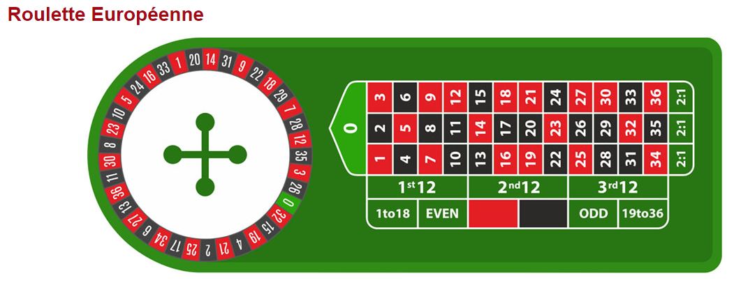
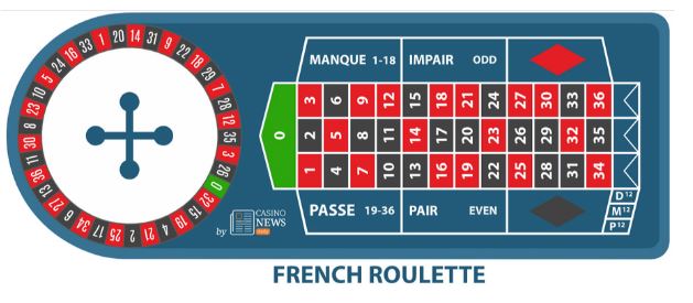
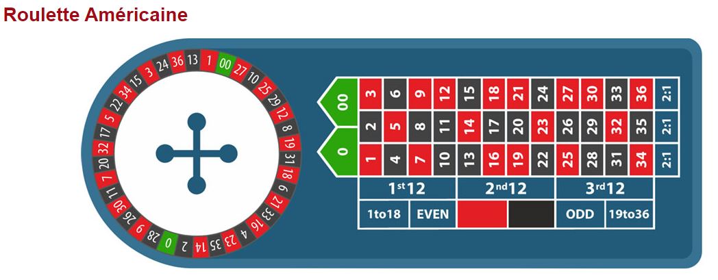
Roulette is a game of chance with several independent players and very limited strategic dimension.
It is generally played by 1 to 9 players, depending on the size of the betting layout.
Equipment :
1. A roulette wheel (or "cylindre") : circular wheel divided into numbered and colored pockets, mounted on an axle allowing free rotation. The wheel can be European or French (37 pockets with a single zero), or American (38 pockets with two zeros).
2. A ball : small sphere intended to circulate in the wheel and settle into one of the pockets when the wheel stops.
3. A betting layout (or table) : flat surface displaying the numbers and types of possible bets, on which players place their wagers.
4. Chips : units used by players to materialize their bets.
Wheel number layout :
In European, French, and American roulette, the exact order of numbers on the wheel, starting from zero and going clockwise, is historical and follows no simple mathematical rule. This order is as follows (see Figures above [BLE][GUI1][GUI2]) :
- European and French roulette (37 pockets with single zero) : 0, 32, 15, 19, 4, 21, 2, 25, 17, 34, 6, 27, 13, 36, 11, 30, 8, 23, 10, 5, 24, 16, 33, 1, 20, 14, 31, 9, 22, 18, 29, 7, 28, 12, 35, 3, 26
- American roulette (38 pockets with 0 and 00) : 0, 28, 9, 26, 30, 11, 7, 20, 32, 17, 5, 22, 34, 15, 3, 24, 36, 13, 1, 00, 27, 10, 25, 29, 12, 8, 19, 31, 18, 6, 21, 33, 16, 4, 23, 35, 14, 2
The number order on the wheel is designed to achieve an optimal balance and ensure game fairness. If the wheel is split in two at the zero :
- Each half contains exactly the same number of reds and blacks.
- Each half contains exactly the same number of evens and odds.
- Each half contains exactly the same number of Manque (1-18) and Passe (19-36).
- Each half contains exactly half of each dozen.
- Each half contains exactly half of each column.
Zeros (0 and 00) are green. The numbers 1 through 36 consist of 18 red and 18 black, arranged in a strictly alternating red/black sequence around the wheel, with no two adjacent numbers of the same color.
For all three variants, colors of numbers 1-36 can be memorized simply : Numbers whose digits sum to odd are red, even are black-with two exceptions : 10 and 28, which are black.
The wheel layout matters little from a probabilistic view point, if the roulette is mechanically perfect and unworn, i.e. without minor balancing flaws or roughness favoring a wheel section. Historically, this arrangement could slightly attenuate local mechanical biases [TOU], but today, with perfectly balanced wheels and rigorous statistical control by casinos, this effect has become practically null.
Spin course :
The goal of the game is to correctly predict the pocket or color where the ball will stop.
A typical spin unfolds as follows :
- The dealer spins the wheel and launches the ball in the opposite direction.
- Players place their bets on the table before the ball settles.
- The ball stops in a pocket.
- Winnings are paid based on the bets.
The dealer [WIK10] :
The dealer is a casino employee. He handles the ball and wheel, records bets, settles player winnings, and announces game phases using traditional formulas :
- "Faites vos jeux" (Make your bets) : start of the betting period.
- "Les jeux sont faits" (No more bets) : ball launch. No new bets accepted.
- "Rien ne va plus" (No more bets) : confirmation of betting closure. Outcome imminent.
- "4 rouge pair et manque" (e.g.) : announcement of winning number and characteristics (color, parity, range).
- "Rien au numéro" (No win on straight Up) : no player won on a Straight Up bet.
- "Rien ne va" (Nothing goes) : ball accidentally left the wheel before settling. Spin canceled and replayed.
Types of bets :
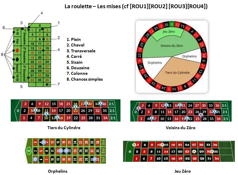
Bets can be classified into three main categories based on their placement on the layout :
- Internal bets (see Figure 1 above, markers 1 to 5) : Bets placed directly on one or more numbers on the layout, covering specific numbers (Straight Up, Split, Street, Corner, Six Line).
- Simple external bets (see Figure 1 above, markers 6 to 8) : Bets placed outside the layout, based on characteristics or regular groups of numbers (color, parity, Low/High, Dozen, Column).
- Special external bets (see Figure 2 above) : Bets announced by the player and made up of several internal bets distributed on the layout by the dealer, covering a specific sector of the wheel (Tiers du Cylindre, Voisins du Zéro, Orphelins, Jeu Zéro).
The following table covers all classic bet types in European (EU), French (FR) and American (US) roulette [WIK10] :
| Bet type | Name | Description | EU/FR/US : Payout (G) | EU/FR : probability (p) | EU/FR : Expectation (E) | US : probability (p) | US : Expectation (E) | Chance Type |
|---|---|---|---|---|---|---|---|---|
| Internal bets | Plein (Straight Up) | Bet on single number | 36 | 1/37 | -1/37 | 1/38 | -2/38 | Multiple Chance |
| Cheval (Split) | Bet on 2 adjacent numbers | 18 | 2/37 | -1/37 | 2/38 | -2/38 | Multiple Chance | |
| Transversale (Street) | Bet on row of 3 numbers | 12 | 3/37 | -1/37 | 3/38 | -2/38 | Multiple Chance | |
| Carré (Corner) | Bet on 4 numbers forming square | 9 | 4/37 | -1/37 | 4/38 | -2/38 | Multiple Chance | |
| Carré "Quatre Premiers" (First Four) | Bet on 4 numbers 0-1-2-3 | EU/FR : 9 | 4/37 | -1/37 | N/A | N/A | Multiple Chance | |
| Sixain (Six Line) | Bet on two adjacent rows (6 numbers) | 6 | 6/37 | -1/37 | 6/38 | -2/38 | Multiple Chance | |
| Five Number Bet | Bet on 5 numbers 0-00-1-2-3 | US : 7 | N/A | N/A | 5/38 | -3/38 | Multiple Chance | |
| Simple external bets | Rouge/Noir (Red/Black) | Bet on pocket color | 2 | 18/37 | -1/37 or FR : -1/74 (La Partage or En Prison) | 18/38 | -2/38 | Simple Chance |
| Pair/Impair (Even/Odd) | Bet on number parity | 2 | 18/37 | -1/37 or FR : -1/74 (La Partage or En Prison) | 18/38 | -2/38 | Simple Chance | |
| Manque/Passe (Low/High) | Bet on 1-18 (Low) or 19-36 (High) | 2 | 18/37 | -1/37 or FR : -1/74 (La Partage or En Prison) | 18/38 | -2/38 | Simple Chance | |
| Douzaine (Dozen) | Bet on 12 consecutive numbers (1-12, 13-24, 25-36) | 3 | 12/37 | -1/37 | 12/38 | -2/38 | Multiple Chance | |
| Colonne (Column) | Bet on one of three vertical layout columns (12 numbers) | 3 | 12/37 | -1/37 | 12/38 | -2/38 | Multiple Chance | |
| Special external bets | Tiers Du Cylindre | Bet covering 12 numbers opposite 0 (6 chips) | EU/FR : Variable depending on the number that comes up (composite bet) | Proportion of numbers covered on the wheel | -1/37 | N/A | N/A | Multiple Chance |
| Voisins Du Zéro | Bet covering 17 numbers around 0 (9 chips) | EU/FR : Variable depending on the number that comes up (composite bet) | Proportion of numbers covered on the wheel | -1/37 | N/A | N/A | Multiple Chance | |
| Orphelins | Bet covering 8 numbers not included in Tiers Du Cylindre or Voisins (5 chips) | EU/FR : Variable depending on the number that comes up (composite bet) | Proportion of numbers covered on the wheel | -1/37 | N/A | N/A | Multiple Chance | |
| Jeu Zero | Bet covering 7 numbers around 0 (4 chips) | EU/FR : Variable depending on the number that comes up (composite bet) | Proportion of numbers covered on the wheel | -1/37 | N/A | N/A | Multiple Chance |
Notes on this table :
1. The payout (G) is the total payout in chips (including the bet), paid by the casino for 1 chip bet (cost c = 1), when the bet is winning. For example, betting 1 chip on a winning Straight Up number returns 35 + 1 = 36 chips.
2. The probability (p) is the probability that a wheel spin results in a total payout G for 1 chip bet.
-
For fixed-payout bets (Straight Up, Simple Chance, Dozen, etc.), p is the physical probability that the winning event occurs.
- For composed bets or special rules (La Partage, En Prison), p can be an effective probability, taking into account partial payouts, neutralizations (zero), or conditional spins.
3. The mathematical expectation (E) is the difference between expected payout (G p) and the cost c : E = (G p) - c
In European/French roulette, and outside the special rules "La Partage" and "En Prison" (see below), we find : E = -1/37 = -0.027, or an average loss of 2.7 % per bet, regardless of (internal or external) bet type.
4. The indication N/A means : Not Applicable
5. Although expectation is identical across bets, distinguishing Simple and Multiple Chances matters for players because :
- Simple Chances offer low payouts but high probability, yielding less spectacular but more frequent wins - ideal for cautious players.
- Multiple Chances offer high payouts but low probability, yielding more volatile wins - suited for bold players.
6. For special external bets, the chip placement on the layout is as follows :
Warning : In some manufacturer wheel printings as well as in photographs used in articles, the number 27 is incorrectly classified among the Orphelins, whereas it actually belongs to the Tiers Du Cylindre.
- Tiers Du Cylindre (6 chips for 12 numbers, see Figure 3 above) : 6 chips, one on each split (5/8, 10/11, 13/16, 23/24, 27/30, 33/36)
- Voisins Du Zéro (9 chips for 17 numbers, see Figure 4 above) : 1 chip on 0 + 8 chips, one on each split (4/7, 12/15, 18/21, 19/22, 32/35), 2 chips on the street (0-2-3), and 2 chips on the corner (25-26-28-29)
- Orphelins (5 chips for 8 numbers, see Figure 5 above) : 1 chip on 1 + 4 chips, one on each split (6/9, 14/17, 17/20, 31/34)
- Jeu Zéro (4 chips for 7 numbers, see Figure 6 above) : 1 chip on 26 + 3 chips, one on each split (0/3, 12/15, 32/35)
7. Standard American roulette differs from European and French roulette by slightly lower probabilities (giving E = -2/38) and an added special bet : Five Number Bet 0-00-1-2-3 (giving E = -3/38). The expectation E increases from -2.7 % to respectively -5.26 % and -7.89 % , making it significantly less favorable for the player.
8. Bet limits, which vary according to bet type and roulette variant, typically range from 1 to 1000 euros for Simple Chances (to satisfy the majority of players) and from 1 to 100 euros for Multiple Chances (to protect the casino's cash reserves in case of very high occasional payouts).
Green numbers :
When the ball lands on a green number (0, or 00 in American roulette), all bets covering 0 win (Straight Up 0, Split 0-1, 0-2, and 0-3, Corner 0-1-2-3, Five Number Bet, Voisins du Zéro, Jeu Zéro). All other bets lose, except for Simple Chances in French roulette when they benefit from the following special rules :
"La Partage" where the player recovers half of their bet, which leads to an expectation E = -1/74 = -1,35 %
Proof : In the non-zero case, the casino pays the player G = 2 (including the bet) with probability 18/37. In the zero case, the casino pays G = 0.5 with probability 1/37. Thus, E = ∑[Gi pi] - c = 36/37 + 0.5/37 - 1 = -1/74
"En Prison" where the bet is held for the next spin and is only lost if that second spin is unfavorable, which leads to an expectation by bet E = -1/74 = -1,35 %
Proof : In the non-zero case, the casino pays the player G = 2 (including the bet) with probability 18/37. In the zero case, and assuming zero does not come up twice in a row, the casino pays G with probability 1/37, where G = 1 with probability 18/36 if the player succeeds on the second spin. Thus, the expected value E per bet = ∑[Gi pi] - c = 36/37 + 1/74 - 1 = -1/74
Warning : Some articles arrive at the erroneous result E = -1/73. The error stems from the arbitrary exclusion of one case out of 74, namely the zero + success case (probability (1/37)(18/36) with G = 1), resulting from a confusion between "net gain = 0" (which is correct) and "actual payment G = 1" (which is wrongly excluded as "not counting" [DEL2]). The biased calculation is : E = 72/73 + 0 - 1 = -1/73 and the correct calculation is : E = 72/74 + 1/74 - 1 = -1/74
General calculation for m consecutive zeros (m ≥ 1) :
We denote : a = 1/37
1. Non-zero case (first spin) : The casino pays the player (bet included) G = 2 with probability 18/37, which gives a contribution : 36 a
2. Consecutive zero cases : If zero comes up k times in a row (with k < m), then the casino pays G with probability ak, G being worth 1 with probability 18 a if the player succeeds on the following spin, which gives a contribution : ak 18 a = 18 ak + 1, for k = 1, 2,..., m - 1
3. Last zero case without continuation : On the m-th zero, the casino pays G with probability am, G being worth 1 with probability 18/36 = 1/2 if the player succeeds conditionally on the following spin (zero excluded), which gives a contribution : (1/2) am
The expected value E for a bet of 1 (cost c = 1) is therefore :
E = 36 a + 18 a2 + 18 a3 + ... + 18 am + (1/2) am - c
Setting : A = 1 + a + ... + am - 2 = (1 - am - 1)/(1 - a) = (1 - am - 1)/(36 a), E can be written as :
E = 36 a + B - 1
with : B = 18 a2 A + (1/2) am = 18 a2 (1 - am - 1)/(36 a) + (1/2) am = a/2
We finally obtain : E = 36 a + a/2 - 1 = 73 a/2 - 1 = -1/74
Conclusion : Whatever the number m of consecutive zeros considered in En Prison mode, the expected value of a unit bet remains exactly equal to E = -1/74, with no approximation whatsoever.
In these two special rules, Simple Chances are not lost entirely or inevitably. The player is thus at an advantage : Expectation improves from -2.7 % to -1.35 % with the rule La Partage or En Prison.
Winning Strategy :
There is no winning strategy at roulette. However, there is an optimal strategy aimed at limiting losses and managing risk, based on the following rules [PER][CHA] :
1. Limit the number of spins : Roulette being a game of chance with negative expectation, the longer you play, the closer average loss converges to theoretical expectation (-2.7 % in European/French roulette). Fewer spins reduce probability of significant losses.
2. Prefer Simple Chances (Red/Black, Even/Odd, Low/High) : All bets have identical negative expectation per spin (-2.7 %), but Simple Chances offer less spectacular but more frequent wins, thereby avoiding abrupt losses. In French roulette, this negative expectation drops to -1.35 % per bet with the rule La Partage or En Prison.
3. Playing so-called "frequent" numbers is an illusion, not due to the layout of numbers on the betting table, but because a mechanical defect localized on a specific pocket of the wheel is extremely unlikely, for two main reasons :
- A worn or defective roulette wheel favors a geographic zone of the cylinder (contiguous sector), not an isolated pocket.
- Casinos monitor, adjust, and replace wheels as soon as a statistical anomaly appears.
4. Palying on the opposite outcome after a series of identical results is also an illusion if one believes that the preceding streak changes the probability of the next spin. For a fair roulette wheel, each spin is indeed independent of the previous ones (for example, P[Odd | a series of Even results immediately beforehand] = P[Odd]) : the ball has no memory, and the probability remains the same on every spin. However, over a longer sequence, subsequent spins statistically tend to reduce the imbalance created by an atypical streak, as the observed frequencies move in the long run toward their theoretical value, without this altering the probability of the next spin.
5. A rational roulette strategy consists of setting an initial bankroll and a stop-loss threshold (e.g., -30 %), with the player psychologically accepting the potential total loss of any gains. It does not alter the game's negative expected value, but allows for serene and prolonged play while limiting losses before they worsen.
B7.6.3. Boule [PER][CHA] :
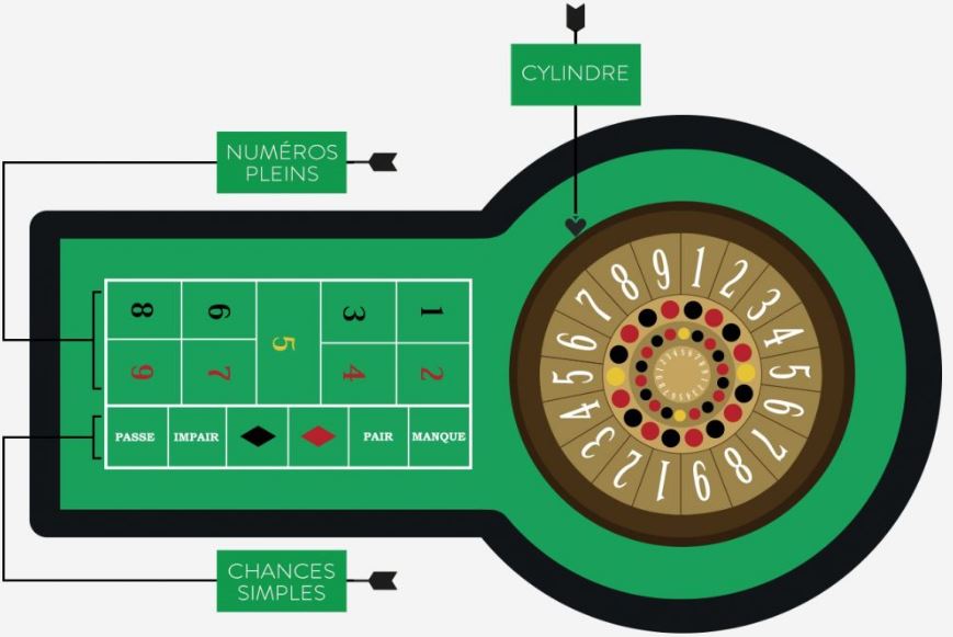
Boule game is a simplified variant of the roulette, using only the numbers from 1 to 9.
It is generally played by 1 to 8 players, depending on the size of the gaming mat.
Equipment :
- A gaming wheel (or "cylindre") : circular wheel divided into pockets numbered 1 to 9 and colored, mounted on an axle allowing free rotation.
- A ball : small sphere intended to circulate in the wheel and settle into one of the pockets when the wheel stops. The ball is a slightly larger ball than the one in roulette in order to fit the larger pockets.
- A gaming layout (or table) : flat surface displaying the numbers and types of possible bets, on which players place their bets.
- Chips : units used by players to materialize their bets.
Wheel number layout :
In casinos, the Boule game is primarily played on an 18-pocket wheel (with two successive series of 1 to 9).
Other versions (such as 27 pockets) exist but are rare and outside the standard framework.
The exact order of numbers on the wheel, starting from 1 and going clockwise, follows a linear sequence 1-2-3-4-5-6-7-8-9 (first sequence) followed by an identical second sequence (see Figure above [BON]) :
Number 1 is black. Reds and blacks numbers then alternate on the wheel, skipping number 5 which is green.
Spin course :
The spin course is identical to that of roulette.
The dealer :
The role of the dealer in the "spinning wheel" version of the Boule game is identical to that of roulette.
Types of bets :
Bets can be classified into two main categories based on their placement on the layout (see Figure above) :
- Internal bets : bets placed directly on one or more numbers on the layout, covering specific numbers (Plein).
- External bets : bets placed outside the layout, based on characteristics or regular groups of numbers (color, parity, Low/High).
The following table covers all classic bet types :
| Type de mise | Nom | Description | Payout (G) | probabilité (p) | Espérance (E) | Type de Chance |
|---|---|---|---|---|---|---|
| Internal bets | Plein (Straight Up) | Bet on single number | 8 | 1/9 | -1/9 | Multiple Chance |
| External bets | Rouge/Noir (Red/Black) | Bet on pocket color | 2 | 4/9 | -1/9 | Simple Chance |
| Pair/Impair (Even/Odd) | Bet on number parity | 2 | 4/9 | -1/9 | Simple Chance | |
| Manque/Passe (Low/High) | Bet on 1-4 (Low) or 6-9 (High) | 2 | 4/9 | -1/9 | Simple Chance |
Note on this table :
1. The payout (G) is the total payout in chips (including the bet), paid by the casino for 1 chip bet (cost c = 1), when the bet is winning. For example, betting 1 chip on a winning Plein number returns 7 + 1 = 8 chips.
2. The probability (p) is the physical probability that a wheel spin results in a total payout G for 1 chip bet.
3. The mathematical expectation (E) is the difference between expected payout (G p) and the cost c : E = (G p) - c
We find : E = -1/9 = -0.111, or an average loss of 11.1 % per bet, regardless of (internal or external) bet type .
4. Although expectation is identical across bets, distinguishing Simple and Multiple Chances matters for players because :
- Simple Chances offer low payouts but high probability, yielding less spectacular but more frequent wins - ideal for cautious players.
- Multiple Chances offer high payouts but low probability, yielding more volatile wins - suited for bold players.
The green number :
When the ball lands on the green number (5), only the Plein bet on 5 wins, and all other bets (Plein 1-4 and 6-9, and Simple Chances) lose.
Winning strategy :
There is no winning strategy for the Boule game. However, there is an optimal strategy aimed at limiting losses and managing risk.
This strategy is identical to that of roulette but with a significantly higher negative expectation (approximately -11 % versus -2.7 %).
In return, Boule is a simpler game, offering quick and intuitive spins.
B7.6.4. Slot machines [PER][CHA] :
Slot machines are individual chance games with very limited strategic dimension.
We mainly distinguish three categories of machines :
- Classic mechanical three-reel machines.
- Modern video machines with digital screens and virtual reels, often five in number.
- Progressive machines, where a portion of bets feeds a shared collective pot between several connected machines.
The rules of the classic three-reel machine are described below.
Equipment (see Figure above) :
1. A machine consisting of three mechanical reels arranged side by side. Each reel bears a specific number of distinct symbols distributed around its circumference. A horizontal payline crosses the reels. The symbols that align on it when stopped determine whether the combination is winning and the associated payout amount.
2. Tokens (or coins) : units used by players to participate in the game.
3. Lever or start button : mechanism activated by the player to trigger the simultaneous rotation of the three reels.
Symbol arrangement on the reel :
Each reel is a cylinder featuring a specific number of successive positions (typically 64), each marked with a standard symbol.
The most common symbols are as follows :
- Cherry : frequent symbol, modest payout.
- Bar (BAR) : less frequent symbol, higher payouts.
- Star or Bell : rare symbols, substantial payouts.
- Number 7 : very rare symbol, often associated with the maximum payout (Jackpot).
- Symbol without payout value (generally white).
The frequency of each symbol's appearance, as well as the payout table associated with the different winning combinations, are defined by the machine manufacturer to ensure a mathematical advantage for the house (casino), typically between 5 % and 10 % of the amounts bet.
Spin procedure :
- Bet : The player inserts 1, 2, or 3 tokens. 3 tokens are required to access the Jackpot.
- Start : The player pulls the lever or presses the button, causing the three reels to spin simultaneously.
- Stop : The reels stop successively. Payouts are awarded only when the three symbols aligned on the central payline are strictly identical. Otherwise, the spin is lost.
- End : The player's bet is permanently consumed. When the obtained combination is winning, the machine dispenses a number of tokens corresponding to the payout specified in the payout table.
Winning conditions :
- The payout amount depends on the obtained combination and the number of tokens bet (1, 2, or 3), according to the payout table.
- The payout table indicates the payout in tokens, paid by the machine for 1 token bet and consumed.
- On a classic three-reel machine, each reel featuring 64 symbols, the payout amounts by combination are given in the following table :
| Combinaison | Number of symboles per reel | Payout (G) | probability (p) |
|---|---|---|---|
| One cherry | c = 16 | 0 | 3 (c/64) ((64 - c)/64)2 = 0,422 |
| Two cherry | c = 16 | 0 | 3 (c/64)2 (64 - c)/64 = 0,0469 |
| Three cherry | c = 16 | 10 | (c/64)3 = 0,0156 |
| Three Bars | b = 8 | 120 | (b/64)3 = 1,95 10 -3 |
| Three Star or Bell | e = 4 | 250 | (e/64)3 = 2,44 10 -4 |
| Three 7 | s = 1 | 800 (Jackpot) | (s/64)3 = 3,81 10-6 |
Notes on this table :
1. Payout (G) is the payout in tokens, paid by the machine for 1 token bet and consumed (cost c = 1), according to the payout table. The G values shown are illustrative but plausible for a classic machine.
2. Probability (p) is the probability that a given combination results in payout G.
For example, the calculation of p for the "One cherry" combination is as follows :
3 = three possible positions for the cherry on the payline (left, center, or right).
(c/64) = probability of getting 1 cherry on the given position.
((64 - c)/64)2 = probability that the 2 other symbols are anything except cherry.
3. Mathematical expectation (E) for a spin is the difference between the expected payout ∑[Gi pi] and the cost c : E_spin = -0.055
On average, for each spin, the player loses approximately 5.5 % of their initial bet.
Winning strategy :
There is no winning strategy on a slot machine, as each spin is independent and governed by chance.
However, there exists an optimal strategy aimed at limiting losses and managing risk.
This strategy is identical to that of the roulette but with a significantly higher negative expectation (approximately -5.5 % vs. -2.7 %).
B7.7. Sports games :
Here are some sports games with or without associated betting.
B7.7.1. French PMU [PER][CHA] :
The French PMU ("Pari Mutuel Urbain") is a horse racing betting game where multiple independent players bet on the same event.
This game allows only limited strategic depth, as horse behavior remains predominant.
Equipment :
1. Official list of runners, published before each race, allowing players to know the numbers, names, jockeys (or drivers), and indicative odds of the entered horses.
2. Betting grid mentioning in the standardized order (see Figure above) :
- Race identification in the grid header : meeting number (corresponding to the hippodrome with date/time) and race number
- Bet type, selected using buttons or checkboxes
- Order/disorder mode, to be checked in specific boxes
- Numbers of the chosen horses on the main grid : boxes numbered 1 to 18
- Amount bet : unit amount (1.50, 2, 3 euros, etc.) or multiples
Example of Quinté+ order grid : [Meeting 1 - R5 Vincennes], [Quinté+], [Order], [Checked numbers : 2-8-11-14-6], [Stake : 2 euros].
3. Type of betting support : either paper ticket (filled manually and validated at an authorized point of sale counter), or digital recording made via an electronic terminal at a point of sale (example : partner tobacco shops), or mobile application or official PMU website (pmu.fr).
Race procedure :
- Start : The race begins with the presentation of the horses to the public and in the paddock (approximately 30 minutes before the start). Betting remains open until official closure, typically 2 to 5 minutes before the actual departure.
- Race : The event, lasting an average of 1 to 5 minutes (flat racing, trotting, or jumping), takes place under the supervision of officials and stewards responsible for enforcing the racing code. At the finish, a provisional ranking is established. In case of a close finish, photo-finish technology determines the order of arrival.
- Final results : Results become final after validation by the stewards, usually within 10 to 20 minutes following the finish, unless there is an objection or investigation. This validation triggers the official publication of odds and initiates payment of winnings to successful bettors.
Winning conditions :
The amount of winnings is proportional to the stake placed and inversely proportional to the total amount of winning stakes recorded on the same bet type.
For each bet type and each race, players' stakes constitute a common pool. After application of regulatory deductions (typically 20 %), the balance is distributed among winning bettors only, pro rata to their stake.
Example :
- Total pool of 100 euros.
- Amount to be distributed R = 80 euros (after 20 % deduction).
- If there are 2 sole winners who staked 1 and 3 euros respectively, the odds r are the ratio between the amount R to be distributed and the sum of winning stakes : r = 80/(1 + 3) = 20
- Each winner then receives an amount equal to stake ratio, i.e. 20 euros for the first player and 60 euros for the second.
- Each player's net gain, after deduction of their initial stake, is therefore 19 and 57 euros respectively.
The following table lists the main bet types offered by PMU, with their theoretical probability of winning (calculated for a race with n = 15 runners).
| Bet type | Description | Average odds (r) | probability (p) | Expectation (E) |
|---|---|---|---|---|
| Simple winner | Exact 1st | 6-12 | 1/n = 1/15 = 6.67 % | -0.60 to -0.20 |
| Simple placed | 1st, 2nd or 3rd | 1-3 | 3/n (for n ≥ 8) = 3/15 = 20.0 % | -0.80 to -0.40 |
| Exacta order | 1st and 2nd in order | 80-200 | 1/(n(n - 1)) = 1/210 = 0.476 % | -0.62 to -0.05 |
| Exacta disorder | 1st and 2nd any order | 25-60 | C(n - 2, 0)/C(n, 2) = 2/(n(n - 1)) = 2/210 = 0.952 % | -0.76 to -0.43 |
| 2 out of 4 | Selection of 4 horses with at least 2 finishing in top 4 | 3-15 | C(n - 2, 2)/C(n, 4) = 78/1365 = 5.71 % | -0.83 to -0.14 |
| Trio order | 1st, 2nd and 3rd in order | 800-1200 | 1/(n(n - 1)(n - 2)) = 1/2730 = 0.0366 % | -0.71 to -0.56 |
| Trio disorder | 1st, 2nd and 3rd any order | 25-40 | C(n - 3, 0)/C(n, 3) = 6/(n(n - 1)(n - 2)) = 6/2730 = 0.220 % | -0.95 to -0.91 |
| Tiercé order | 1st, 2nd and 3rd in order, with possible rollover | 800-2500 (no bonus B) 50-200 (with avg B = 0.08 %) | 1/(n(n - 1)(n - 2)) = 1/2730 = 0.0366 % + avg B = 0.12 % | -0.71 to -0.084 -0.067 to +1.92 |
| Tiercé disorder | 1st, 2nd and 3rd any order, with possible rollover | 80-300 (no bonus B or avg B = 0.25 %) | C(n - 3, 0)/C(n, 3) = 3!/(n(n - 1)(n - 2)) = 6/2730 = 0.220 % + avg B = 0.47 % | -0.82 to -0.34 -0.62 to +0.41 |
| Quarté+ order | 1st to 4th in exact order, with possible rollover | 10000-80000 (no bonus B or avg B = 0.15 %) | 1/(n(n - 1)(n - 2)(n - 3)) = 1/32760 = 0.00305 % + avg B = 0.153 % | -0.70 to +1.4 +14.3 to +121.4 |
| Quarté+ disorder | 1st to 4th any order, with possible rollover | 1000-15000 (no bonus B or avg B = 0.30 %) | C(n - 4, 0)/C(n, 4) = 4!/(n(n - 1)(n - 2)(n - 3)) = 24/32760 = 0.0732 % + avg B = 0.301 % | -0.27 to +10.0 +2.0 to +44.2 |
| Quinté+ order | 1st to 5th in exact order | 80000-300000 | 1/(n(n - 1)(n - 2)(n - 3)(n - 4)) = 1/360360 = 0.00028 % | -0.78 to -0.16 |
| Quinté+ disorder | 1st to 5th any order, with possible rollover | 2500-25000 (no bonus B or avg B = 0.11 %) | C(n - 5, 0)/C(n, 5) = 5!/(n(n - 1)(n - 2)(n - 3)(n - 4)) = 120/360360 = 0.0333 % + avg B = 0.143 % | -0.17 to +7.3 +2.6 to +34.8 |
| Tic 3 | Selection of 5 horses allowing simultaneous play on Tiercé, Quarté+ and Quinté+ disorder | 15-80 | C(5, 3)/C(n, 3) + C(5, 4)/C(n, 4) + C(5, 5)/C(n, 5) = 10/455 + 5/1365 + 1/3003 = 2.60 % | -0.61 to +1.08 |
Notes on this table :
1. The odds (r) are the final ratio (euros won per euro staked), published after the race.
2. The probability (p) is the purely combinatorial probability of winning the bet, assuming each horse is equiprobable.
Binomial coefficient C(a, b) = a!/(b!(a - b)!)
3. The Bonus B is the additional probability of the bet in case of pool rollover when no player wins the bet (redistribution of stakes to extended positions of the same race : 4th, 5th, etc., for Tiercé for example).
4. The mathematical expectation (E) of a unit stake bet (cost c = 1) is the difference between the expected winnings (c r) p and the cost c.
Example : For a c = 1 euro stake on Simple Winner with historical average odds r = 10, and n = 15 runners, E = (1 10) 1/15 - 1 = -0.33 euro, i.e. an average loss of 33% per euro staked.
The mathematical expectation E shows an average loss of 30 to 60 % across all bet types, but can exceptionally approach zero, particularly on Tiercé, Quarté+, or Quinté+ during significant rollovers.
Winning strategy :
There is no winning strategy for French PMU betting, but there exists a rational strategy aimed at reducing losses.
The expectation E is positive if and only if the odds r exceed the critical threshold 1/p. Consequently, the rational strategy is as follows [PER][CHA] :
- Target bets where the estimated pre-race odds (r) are very close to the critical threshold 1/p from the previous table.
- Identify underbet favorites (horses with high actual win probability but lightly bet, thus offering high odds r).
- Avoid bets on heavily oversubscribed pools (too many bettors on one horse).
- Diversify stakes across multiple bet types.
- Do not consider Tiercé, Quarté+, or Quinté+ bets as inherently preferable due to potential bonuses, as bonus situations remain statistically exceptional.
- For simple bets (single horse), avoid market extremes (overbet favorite and speculative longshot) and favor intermediate horses (2nd or 3rd favorites).
- For compound bets (multiple horses), build balanced combinations, often around a solid favorite, adding underbet intermediate horses.
B7.7.2. Soccer [PER][CHA] :
Soccer is a team sport pitting two teams of eleven players against each other on a field, aiming to score goals by propelling a spherical ball, primarily with the feet.
This game features a significant strategic dimension where collective tactics and individual qualities play an essential role.
Equipment :
- Field (see Figure above) : Rectangular area (length 90-120 m x width 45-90 m) with corner flags (minimum height 1.5 m), two goals with nets (width 7.32 m x height 2.44 m), penalty area in front of each goal (depth 16.5 m x width 40.32 m), goal lines, touchlines, halfway line.
- Ball : Spherical, circumference 68-70 cm, weight 410-450 g, pressure 0.6-1.1 atm.
- Players : 11 per team (10 outfield players + 1 goalkeeper), with mixed teams allowed in non-specific categories.
- Equipment : Numbered jersey, shorts, socks, shin guards mandatory, studded boots, distinct kit for the goalkeeper, jewelry prohibited.
Objective :
- Objective : Score more goals than the opposing team by propelling the ball into the opponent's goal, primarily with the feet (head and torso allowed).
- Duration : 90 minutes (2 x 45 min. with 15-min. halftime), extra time in case of tie (2 x 15 min. in knockout stages) and penalty shootout if necessary.
- Penalty shootout : If the tie persists after extra time, a session of 5 alternating penalties. If the tie remains, the session continues shot by shot in sudden death.
- Sudden death : As soon as one team leads and the other misses its corresponding shot.
Kick-off :
Kick-off : Ball at the center of the field, drop kick (drop consisting of releasing the ball from the hands and striking it with the foot after the bounce), either at the start of the match by the home team (or by toss) or by the team that did not score the last goal.
Other restarts :
- Throw-in : Ball gone out over the touchline, thrown in with two hands from the point of exit by an opponent.
- Goalkeeper clearance : Ball gone out over the goal line, last touched by a teammate, restarted by the goalkeeper from the penalty area.
- Corner : Ball gone out over the goal line, last touched by an opponent, kicked from the nearest corner.
- Free kick direct or indirect.
Fouls :
Direct free kick (or penalty if committed in own penalty area) :
- Violent charge : Excessive physical contact with an opponent.
- Dangerous tackle : Excessive use of feet or legs.
- Spitting : Projecting saliva at any person.
- Deliberate handball : Intentional touching of the ball with hand or arm (except goalkeeper in penalty area).
- Holding or pushing an opponent : Action with hands or body.
- Violent conduct against an opponent, even without contact.
Indirect Free Kick :
- Offside : A player located in the opponent's half of the field, nearer to the goal line than both the ball and the second-to-last opponent, at the moment a teammate plays the ball toward him (pass, cross, etc.). No offside if the player is in his own half, directly controls the ball (dribble, first touch), or if the ball comes from a throw-in, corner, or goal kick.
- Dangerous play without contact : Risky action without touching the opponent (e.g., foot raised to head height).
- Impeding without contact : Blocking an opponent without playing the ball.
- Simulation : Exaggerated dive to deceive the referee.
- Back-pass to goalkeeper : On a deliberate foot pass from a teammate, the goalkeeper may play the ball but not with hands.
- Goalkeeper double contact : If the goalkeeper releases the ball from hands, he cannot pick it up again until another player has touched it.
- Goalkeeper's 6 seconds : Goalkeeper holding the ball longer than 6 seconds.
- Antisporting behavior with goalkeeper : Repeated or unnecessary use of the goalkeeper to circulate the ball and waste time.
Sanctions :
- Yellow card : Warning (2 yellows = red).
- Red card : Immediate expulsion (serious foul, violent conduct, or accumulation of two yellow cards).
- Penalty : Single shot from the penalty spot (11 m), with only the goalkeeper as opponent.
Winning strategy :
The main rules aimed at dominating the opponent are as follows :
Defensive strategies :
- Collective pressing : Upon loss of possession, the team quickly repositions to apply pressure and slow down the opponent's progression.
- Zonal marking : Each player covers a specific zone rather than an individual opponent, reducing risks of simulation or obstruction.
- High defensive line : The defense positions itself advanced to trap attackers in offside positions.
Offensive strategies :
- Quick transitions : Upon ball recovery, immediately launch a counter-attack to exploit spaces left by the opponent.
- Short combinations : Use precise short passes to destabilize the opposing defense and create exploitable gaps.
- Wing play : Develop play on the flanks with overlaps and crosses to provoke corners or penalties.
Match management :
- Possession mastery : Keep the ball as long as possible with precise build-up play.
- Dominance periods management : Capitalize on periods of control to score, anticipating extra time and penalties if necessary.
- Foul exploitation : Provoke direct fouls from opponents to obtain yellow cards and strategic free kicks.
B7.7.3. Rugby union [PER][CHA] :
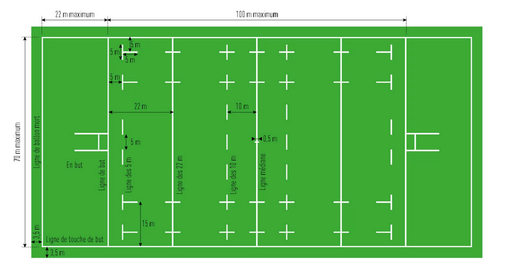
Rugby union is a team sport pitting two teams of fifteen players against each other on a field, aiming to score points, particularly by grounding an oval ball in the opponent's in-goal area for a try, primarily with the hands.
This game features a significant strategic dimension where collective tactics and individual qualities play an essential role.
Equipment :
- Field (see Figure above) : Rectangular area (width 68-70 m x length 94-100 m between goal lines), two H-shaped posts (spacing 5.6 m, crossbar at 3 m height) on each goal line, an in-goal area behind each goal line (width 68-70 m x depth 10-22 m), goal lines, touchlines, dead-ball lines, 22 m lines, halfway line.
- Ball : Oval, length 28-30 cm, circumference (long axis) 74-77 cm, weight 400-440 g, pressure 0.66-0.75 atm.
- Players : 15 per team (8 forwards + 7 backs), with substitutes (up to 8 in official competition).
- Equipment : Numbered jersey, shorts, socks, studded boots, mouthguard mandatory, soft protections allowed (helmet, shoulder pads, etc.), distinct kit for each team.
Objective :
- Objective : Score more points than the opposing team by grounding the ball in the opponent's in-goal area (try or by kicking the ball between the posts (conversion after try, penalty, drop goal), primarily with the hands.
- Duration : 80 minutes (2 x 40 min. with 10-15 min. halftime), extra time in case of tie (2 x 10 min. in knockout stages) and sudden death if necessary.
- Sudden death : The first scoring points decide the winner.
Kick-off :
Kick-off : Ball at the center of the field, dropped from hands and kicked after bounce (drop kick), either at the start of the match by the team drawn by lot, or by the team that did not score the last points (try, conversion, penalty, or drop goal).
Other restarts :
- Line-out : Ball gone out over the touchline, thrown in with two hands overhead from the point of exit by a player from the opposing team.
- Scrum : After certain minor infringements, 8 players from each team bind together to contest the ball introduced into the tunnel by the scrum-half.
- Penalty : After an opponent's foul, the benefiting team may choose: attempt the goal, kick to touch, play quickly by hand, or opt for a scrum.
- 22-meter drop-out : When the ball is made dead or grounded in the defending team's in-goal (the team not in possession) without a try being awarded, that team restarts with a drop kick from its own 22-meter line.
- Ruck : After a tackle with the ball on the ground, players from both teams bind upright over the ball to contest it with their feet.
- Maul : The ball carrier is held upright by an opponent and pushed forward by teammates to advance.
Scoring table :
Try (ball grounded in the opponent's in-goal area) : 5 pts
Conversion after try (place kick or drop, with ball passing between the posts) : 2 pts
Penalty (place kick with ball passing between the posts) : 3 pts
Drop goal (drop with ball passing between the posts) : 3 pts
Penalty try : 7 pts (5 + automatic conversion granted)
Fouls :
Penalty :
- Dangerous tackle : Tackle above the shoulders.
- Illegal tackle : Tackle without wrapping (e.g., from behind).
- Obstruction : Blocking an opponent without playing the ball.
- Offside : Player ahead of his ball-carrying teammate or in a prohibited position.
- Hands in ruck : Handling the ball in a formed ruck.
- Holding opponent : Grasping an opponent without attempting to play the ball.
Penalty try :
- Violent blows : Punch, deliberate kick.
- Dangerous conduct : Shoulder to face, head-first tackle.
Free kick :
- Minor offside : Irregular position in static phase (scrum, line-out, open play).
- Irregular scrum introduction.
- Irregular line-out (e.g., crooked throw).
Sanctions :
- Yellow card : Temporary player exclusion (10 minutes). The team plays with 14 players during the sanction.
- Red card : Permanent player expulsion for the rest of the match (serious foul, violence, or two yellow cards) with no replacement possible.
- Penalty.
Winning strategy :
The main rules aimed at dominating the opponent are as follows :
Defensive strategies :
- Collective pressing : Upon loss of possession, the team quickly repositions to apply pressure and slow down the opponent's progression.
- Aligned defense : Organized and compact defensive line to close central spaces and channel the attack toward the flanks.
- Ruck contestation : Legal pressure on ruck phases to attempt ball recovery or slow down the release.
Offensive strategies :
- Penetrating play : Straight runs by forwards to pin the defense and create gaps.
- Wide play : Use of passes to stretch the defense and exploit spaces on the wings.
- Rolling maul : Forwards bound together pushing the carrier to gain meters through successive phases.
Match management :
- Scrum mastery : Use scrums to secure possession and structure attacks.
- Dominance periods management : Convert periods of control into points.
- Penalty exploitation : Choose the best option based on field position.
B7.8. Sources relating to Strategy games
[BLE] Bleach-Mx, Comment fonctionne la roulette française ?.
[BON] Bonus Roulette, COMMENT JOUER AU JEU DE LA BOULE AU CASINO ?.
[CHA] ChatGPT, le moteur d'Intelligence Artificielle développé par OpenAI.
[CUR] Courses de vecteurs, Course de vecteurs.
[DEL1] Jean-Paul Delahaye, Stratégies magiques au pays de Nim, Pour la Science - n 377 - Mars 2009.
[DEL2] Jean-Paul Delahaye, Les martingales et autres illusions, Pour la Science - n 251 - Septembre 1998.
[GUI1] Guide Roulette, Roulette Européenne.
[GUI2] Guide Roulette, Roulette Américaine.
[JEU] Jeux Solo ici et là, ACCORDEON #31 (Youtube, 11:54).
[PER] Perplexity, le moteur d'Intelligence Artificielle développé par Perplexity AI.
[ROU1] Roulette 17, Tiers Du Cylindre.
[ROU2] Roulette 17, Voisins Du Zero.
[ROU3] Roulette 17, Orphelins.
[ROU4] Roulette 17, Jeu Zero.
[TOU] Pierre Tougne, Roulette, Loto et probabilités, La mathématique des jeux, pp.147-156, Pour la Science, 1991.
[TRI1] Jean Tricot, Jeux et informatique - Le jeu des pièces de 10 francs, Science et Vie - n 722 - Novembre 1977.
[TRI2] Jean Tricot, Jeux et informatique - Le jeu de Northcott, Science et Vie - n 724 - Janvier 1978.
[WIK1] Wikipedia, Bataille (jeu).
[WIK2] Wikipedia, Bataille navale(jeu).
[WIK3] Wikipedia, Racetrack (game).
[WIK4] Wikipedia, Crapette.
[WIK5] Wikipedia, Yahtzee.
[WIK6] Wikipedia, Pig (dice game).
[WIK7] Wikipedia, Morpion (jeu).
[WIK8] Wikipedia, Tic-tac-toe.
[WIK9] Wikipedia, Poker.
[WIK10] Wikipedia, Roulette (jeu de hasard).
 Last page update : June 24, 2026.