| En Français | Home/Contact | Billiards | Hydraulic ram | HNS | Relativity | Botany | Music | Ornitho | Meteo | Help |
This page gives the basic formulas of Restricted Relativity and General Relativity with a presentation of the mathematical tools accessible to uninitiated people.
This page also includes a detailed Lexicon of terms used in Relativity.
Notations on this page :
- The keywords have their first letter indicated in uppercase and are defined in the Lexicon.
- The authors quoted are referenced in square brackets under the reference [AUTHOR Title Page]. See Bibliography.
- The Mathematical notations are consistent with rare exceptions to those of Eric Gourgoulhon, Research Director at the CNRS [GOU, Relativité Restreinte][GOU, Relativité Générale].
- The Sign conventions are classically those of Misner, Thorne and Wheeler (MTW), with a Metric tensor of Signature (-, +, +, +), a Curvature tensor defined by Rijkl = Γijl,k + .. ., and a Ricci tensor defined by Rij = Rkikj
The relativity idea does not date from Einstein but finds its origin in the Galileo works.
We consider two Observers in relative motion whose reference frames are in rectilinear translation with uniform speed with respect to each other. These reference frames are called inertial.
Today there remains one final challenge : the unification of General Relativity and Quantum theory in order to make coherent the gravitation on a macroscopic scale and the gravitation on a microscopic scale involving the quantum character of the elementary particles.

The time relativity, whether in Restricted or General Relativity, encompasses two distinct phenomena that are often confused :
- Simultaneity relativity
- Multiplicity of proper times
1.2.1. Simultaneity relativity :
Events that are simultaneous for one observer may not be simultaneous for another observer in relative motion to the first.
This real phenomenon is not mysterious in itself because it logically results from the light speed which is finite, combined with the invariance of the light speed in all inertial reference frames with respect to the movement of the light source and the observer.
"On a human scale, the light speed is prodigiously high (about 300 000 km/s). When a light source emits a signal, the light gives us an almost instantaneous information. We believe to see the space at a given moment. Time seems absolute, separated from space." [AND Théorie - Partie 1]
Imagine two Observers O and O' in relative movement with respect to each other, who wish to set their watches by exchange of optical signals. Suppose that the two watches are synchronized by any means so that they indicate the same time at the same initial instant. At this instant each Observer sends a signal to the other. What time does each watch indicate when each Observer receives the signal from the other ? It is obvious that this is not the same time.
And Poincaré explains : "The transmission duration is not the same in both directions since the Observer O, for example, goes ahead of the optical propagation emanating from O', while the Observer O' flees the propagation emanating from O. The watches will indicate what can be called local time of each Observer, so that one of them will delay on the other. It does not matter since we have no way of seeing it..." [POI L'Etat, p.311]
The indicated time is the same for both Observers only in the case of Observers fixed with respect to each other or in the thought hypothesis of a light having an infinite speed. In other cases, we speak of apparent durations dilation.
Thus, the instant universe is unobservable. It appears as a Space-time where each observed object is seen at a space point and at a time point that is not the same for all space points." [AND Théorie - Partie 1]
1.2.2. Multiplicity of proper times :
The proper time measured by an observer stationary in his reference frame is unique to that observer. Two observers in relative motion to each other, or subject to different gravitational fields, will accumulate different proper times even if they find themselves at the same point in space-time.
This real phenomenon remains mysterious to this day and results from the properties of space-time concerning both :
1. the relative movement of observers (principle of Restricted Relativity).
2. the presence of gravitational fields (physical deformation of space-time).
The theory of Relativity, although mathematically consistent and experimentally verified, does not always provide intuitive explanations of the phenomena it describes. The Multiplicity of proper times is one of them, illustrating the limits of our intuitive understanding of the universe on a large scale. [PER]
Added to this are some clumsiness that do not facilitate the reading and understanding of Relativity. We can list :
|
Before reading a book on Relativity, it is therefore prudent to check at least : - The presence or not of an index of notations used, which greatly facilitates the reading of the book. - The vector notation used, making it possible to distinguish unambiguously between scalar, vector and tensor quantities. - Any writing simplifications, in particular the arbitrary setting to 1 of speed of light (c), universal gravitational constant (G) and/or dielectric permittivity in vacuum (ε0). - The sign conventions used, in particular if they are identical or not to the classic MTW sign conventions, namely : a Metric tensor of Signature (-, +, +, +), a Curvature tensor defined by : Rijkl = Γijl,k + ..., and a Ricci tensor defined by : Rij = Rkikj. For these three classic conventions, Einstein Field Equation must be strictly the following : Rab - (1/2) gab R + Λ gab = K Tab - The metric used, in particular that of Minkowski (Restricted Relativity), that of Schwarzschild (astronomy of General Relativity) or that of Friedmann-Lemaître-Robertson-Walker (cosmology of General Relativity). |
Einstein's postulate states that the light speed in a vacuum is invariant in all inertial reference frames with respect to the motion of the light source and the observer.
This invariance postulate is not strictly necessary from a mathematical point of view and can be replaced by the causality postulate which is more general and less artificial [SEM]. The latter indeed shows in fact that there is a limiting speed of propagation of interactions (space-time structure constant) without necessarily specifying that this speed is that of light.
However, although mathematically equivalent, these two postulates offer different perspectives on the physical interpretation of the Relativity theory.
Einstein's postulate is more specific, explicitly identifying the light speed as the limiting speed. This postulate, combined with the principle of Restricted Relativity, gives the principle of invariance of the light speed.
Consequently :
- The light speed is only a specific manifestation of this limit within the framework of electromagnetism.
- The hypothetical questioning of the light speed in vacuum as an absolute limit is not necessarily a questioning of the theory of Restricted Relativity.
- The causality postulate could apply even in situations where light would not play a central role, for example in some theories of quantum gravity.

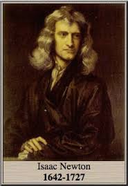

- Until the end of the 19th century, classic mechanics founded by Galileo and Newton constituted an undisputed basis of physics.
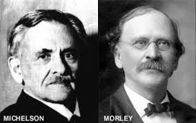
- In 1887 an American physicist Albert Michelson and his colleague Edward Morley showed that the light speed did not verify the Galilean law of addition of velocities. On the contrary, the light speed in the vacuum was independent of the motion of the emitting source.
- At the end of the 19th century, a second enigma disrupted the certainties of the scientists. The famous equations of British James Clerk Maxwell which describe all the phenomena of electromagnetism no longer have the same form when they are transposed from one reference system into another by an uniform rectilinear translation.
Should not the Galilean principle be, if not abandoned, at least rehabilitated ?
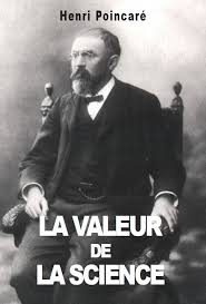
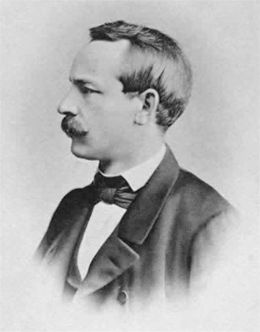
- In 1905 Jules Henri Poincaré laid the fundamental foundations of Restricted Relativity which erased at once all the anxieties of physicists about these two enigmas [POI L'Etat].
He shows that the true basis of Restricted Relativity is the Lorentz-Poincaré transformation which generalizes that of Galileo to speeds not negligible compared to that of light.
- Also in 1905, Albert Einstein published his theory of Restricted Relativity [EIN Zur_Elektrodynamik].
It is also based on the Lorentz-Poincaré transformation but according to a physical interpretation different from that of Poincaré : Restricted Relativity is based on the relative speed of two objects and not their speed relative to an absolute reference frame (the ether).
- This transformation opens the way to revolutionary concepts that were then experimentally verified. We can cite :
1932 : Invariance of the light speed (suggested in 1887 by Michelson & Morley by showing that the luminiferous ether does not exist, then postulated in 1905 by Albert Einstein, then demonstrated in 1932 by Roy Kennedy and Edward Thorndike by verifying that the light speed is independent of the motion of the source).
1930-1950 : Relativistic composition of speeds (indirectly validated by many laboratories in particle accelerators).
1938 : Dilation of durations (demonstrated by Herbert Ives and G.R. Stilwell by measuring the Doppler shift of light emitted by fast-moving ions).
1941 : Lengths contraction (demonstrated indirectly by Bruno Rossi and David B. Hall via the cosmic muon experiment).
1971 : Multiplicity of proper times (confirmed by Hafele & Keating with atomic clocks on board planes flying around the world).
2008 : Mass-energy equivalence (indirectly confirmed in the 1930s-1940s by numerous experiments in nuclear and particle physics, then confirmed in 2008 by the international team of the "Centre de Physique Théorique de Marseille" by showing that the mass of the proton comes from the energy of quarks and gluons).
2011 : Relativistic aberration of light (demonstrated directly by Daniel Giovannini's team at the University of Glasgow, in a terrestrial laboratory).
Note some surprising conclusions among others :
- If two luminous particles move away from each other, their relative speed is equal to c and not 2c (speeds composition law, see below).
- Since the light speed is slowed down in various media according to their refractive index n, it is possible to accelerate particles that go faster than light in the same medium.
Hendrik Antoon Lorentz gave an imperfect version of this tranformation in 1899 and then 1904. Jules Henri Poincaré published the correct equations in 1905, baptizing them with the name of Lorentz.
Warning : This transformation applies exclusively to reference frames in uniform rectilinear relative motion, known as inertial frames. It does not cover accelerated or rotational cases, which are subject to extended (non-inertial) formalisms or General Relativity.
Hypotheses :
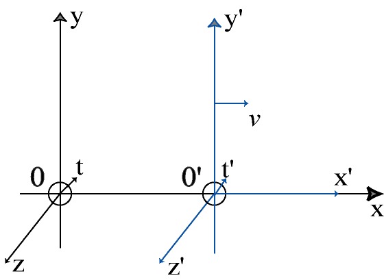
Initially, two orthonormal reference frames R and R' have their origins O and O' coincident at t = t' = 0, with their axes x and x', y and y', z and z' respectively parallel.
Then, the reference frame R' performs a uniform rectilinear translation with respect to R at a constant speed v, measured in R and in the positive direction of the axis x.
Let M be an arbitrary point or event having spatio-temporal coordinates (x, y, z, t) in R and (x', y', z', t') in R'.
The transformation of Galileo from R to R' can be written as follows :
|
(G1) x' = x - v t ; y' = y ; z' = z (G2) t' = t |
The transformation of Lorentz-Poincaré introduces a new entity to describe the physical phenomena : Space-time. This conception unifies space and time into a single four-dimensional structure, explaining in particular the following two phenomena :
1. Apparent contraction of lengths : The length of a moving object relative to an observer appears contracted in the direction of motion when measured by that observer. The dimensions of the object perpendicular to the motion are not affected. This phenomenon is symmetrical : each observer sees the objects in the other reference frame contracted in the direction of motion.
2. Apparent dilation of durations : The time interval between two events occurring at the same location in a given reference frame appears longer when measured from a reference frame in motion relative to the first. This phenomenon is symmetrical : each observer sees the durations in the other reference frame lengthening.
The corresponding equations are written as :
|
(L1) x' = γ (x - v t) ; y' = y ; z' = z (L2) t' = γ (t - B x) (L3) γ = 1 / (1 - v2 c-2)1/2, called Lorentz factor (L4) B = v/c2 |
where c is a constant (Space-time structure constant) which is similar to a limiting speed and which appears during the presentation of the equations (L). The constant c is taken equal to the highest speed currently measured which is that of electromagnetic phenomena in vacuum, in this case the light speed in vacuum.
The inverse transformation consists of replacing v by -v in relations (L1) to (L4) :
|
(L1') x = γ (x' + v t') ; y = y' ; z = z' (L2') t = γ (t' + B x') |
When the velocity v has any direction with respect to the x axis, the transformation of Lorentz-Poincaré is written in vector form as follows (by noting r = (x, y, z) and r' = (x', y', z')) :
|
(LL1) r' = r + (γ - 1) (v.r / v2) v - γ v t (LL2) t' = γ (t - v.r / c2) (LL3) γ = 1 / (1 - v2 c-2)1/2 Proof of the relation (LL1) : The positions r and r' can each be decomposed into two vector components, respectively parallel and perpendicular to the direction of the velocity v : r = rpar + rper r' = r'par + r'per with : rpar = projection of r on the direction parallel to v = (v.r / v2) v rper = projection of r on the direction perpendicular to v = r - rpar The relations (L1) can then be generalized in the form : r'par = γ (rpar - v t) ; r'per = rper Hence the general result : r' = γ (rpar - v t) + rper which can also be written as : r' = r + (γ - 1) (v.r / v2) v - γ v t Proof of the relation (LL2) : The relation (L2) can be generalized in the form : t' = γ (t - rpar.v / c2) We also have the identity : r.v = rpar.v Hence the general result : t' = γ (t - v.r / c2) |
When v is parallel to the x-axis and in the same direction, we have v = (v, 0, 0) and r = (x, y, z), hence: v.r = v x
The relation (LL1) projected on the x-axis becomes : x' = x + (γ - 1) x - γ v t = γ (x - v t)
The relation (LL1) projected on the y-axis becomes : y' = y
The relation (LL1) projected on the z-axis becomes : z' = z
The relation (LL2) becomes : t' = γ (t - v x / c2)
We find the standard relations (L1) to (L4).
When v and r are parallel, we have r = r (v/v) and relations (LL1)(LL2) become : r' = γ (r - v t) (v/v) and t' = γ (t - v r / c2)
Thus, the position r remains unchanged in direction but is modified in magnitude as a function of the velocity v and the time t. Similarly, the time t is modified as a function of the velocity v and the position r.
When v and r are perpendicular, we have v.r = 0 and relations (LL1)(LL2) become : r' = r - γ v t and t' = γ t
Thus, the position r remains unchanged but undergoes an additional displacement ( - γ v t ) in the direction of motion. The time t is simply increased by a factor γ, without any dependence on the position.
The two previous cases highlight the following points :
- The more pronounced space-time interlacing in the parallel case.
- The relative simplicity of the transformation in the perpendicular case.
- In 1975 Jean-Marc Levy-Leblond published an article on Restricted Relativity presented in a modern form deduced only from the properties of space and time, without need for reference to electromagnetism [LEV].
- In 2001 Jean Hladik published, with one of his colleagues Michel Chrysos, the first book in French on Restricted Relativity presented in this modern form, titling these properties "Poincaré's postulates" [HLA Pour_comprendre].
The main conclusions are then as follows :
- The four postulates of Poincaré suffice to single out the Lorentz-Poincaré transformation and its degenerate Galilean limit as the only possible inertial transformations [LEV].
Inspired by the works [LEV][HLA, Pour_comprendre][HLA, Initiation][CAS][SEM], we present below a complete presentation of the Lorentz-Poincaré transformation only based on the four Poincaré's postulates.
|
Proof : Postulat 1 : Space is homogeneous and isotropic Space has the same properties at every point and in every direction. In other words space is invariant by translation and rotation. Postulate 2 : Time is homogeneous The time is identical in every point of the same reference frame. All fixed clocks in a given reference frame must be strictly set at the same time. In other words time is invariant by translation. Postulate 3 (Principle of Restricted Relativity) : The laws of physical phenomena must be the same either for a fixed Observer or for an Observer entrained in an uniform rectilinear translational movement. The form of the equations which describe the mechanical phenomena is invariant by reference frame change by uniform rectilinear translation. Postulate 4 : Causality must be respected When a phenomenon A is the cause of a phenomenon B, then A must occur before B in any reference frame. The desired transformation can be written in the following general form linking the coordinates x and t : x' = F(x, t, v) t' = G(x, t, v) with the following initial conditions : 0 = F(0, 0, v) 0 = G(0, 0, v) Any interval of transformed coordinates can therefore be written as follows : dx' = (dF/dx)dx + (dF/dt)dt dt' = (dG/dx)dx + (dG/dt)dt If space and time are assumed homogeneous, the transformation does not depend on where the is the transformed interval, nor from the epoch to the which the interval is transformed. The coefficients in front of dx and dt are therefore not a function of x and t. Hence for example : dF/dx = F1(v) The two previous relationships are therefore integrated as follows : x' = F1(v) x + F2(v) t + constant t' = G1(v) t + G2(v) x + constant and are simplified as follows, taking into account the two previous initial conditions : (Ha) x' = F1(v) x + F2(v) t (Hb) t' = G1(v) t + G2(v) x where the four functions F1, F2, G1 and G2 are to be determined. The postulates of homogeneity of space and time therefore induce that the desired transformation is linear. The particular point M = O' correspond to : x' = 0 and x = v t Equations (H) can be rewritten as follows : (C1a) x' = γ (x - v t) (C1b) t' = γ (A t - B x) The unknowns become γ, A and B which are three functions dependent only of v. Namely : γ = γ(v) ; A = A(v) ; B = B(v). When v = 0 we must have : x' = x and t' = t corresponding to the identity transformation and it can be deduced that : (C2) γ(0) = 1 The postulate of space isotropy induces that the form of the equations is invariant by reflection (x --> -x ; x' --> -x' ; v --> -v) corresponding to the passage of the " -R " reference frame to the " -R' " reference frame. From this it can be deduced that : (C3a) γ(v) = γ(-v) (C3b) A(v) = A(-v) (C3c) B(v) = - B(-v) The postulate of form invariance induces that the form of the equations is invariant by inverse transformation (x' <--> x ; t' <--> t ; v <--> -v) corresponding to the exchange of the reference frames R and R'. From this it can be deduced that : (C4a) x = γ(-v) (x' + v t') (C4b) t = γ(-v) (A(-v) t' - B(-v) x') From relations (C1)(C3) it can be deduced that : (C5a) A = 1 (C5b) γ2 (1 - v B) = 1 It remains to determine the unknown B. The postulate of form invariance induces that the form of the equations is invariant by composition of the transformations (R --> R') and (R' --> R"). From relation (C5a) it can be deduced that : (C6a) x" = γ(u) (x' - u t') (C6b) t" = γ(u) (t' - B(u) x') where u is the uniform rectilinear translation speed of R" with respect to R', measured in R' and in the positive direction of the axis x' Let w be the uniform rectilinear translation speed of R" with respect to R, measured in R and in the positive direction of the axis x From relation (C1) it can be deduced that : (C7a) w = (v + u) / (1 + u B) (C7b) B(u) / u = B(v) / v The relation (C7a) is the speeds composition law. The relation (C7b) shows that B is of the form : (C8) B(v) = b v where b is any constant (negative, zero or positive). From particular relation (C2) the relation (C5b) can be written : (C9) γ2 = 1 / ( 1 - b v2) with γ > 0 From relations (C5b)(C8)(C9) the equations (C1) can be written : (C10a) x' = (x - v t) / (1 - b v2)1/2 (C10b) t' = (t - b v x) / (1 - b v2)1/2 (C10c) b v2 < 1 It remains to determine the unknown b. Let M1 and M2 be two any points of the reference frame R. From relation (C10b) it can be deduced that : (t2' - t1')/(t2 - t1) = ( 1 - b v ((x2 - x1)/(t2 - t1)) ) / (1 - b v2)1/2 The postulate of causality induces that the sign of the time interval (t2 - t1) in R must not change during the passage in (t2'- t1') in R'. This can be written : (C11) b v (x2 - x1)/(t2 - t1) < 1 If b is zero, the relation (C11) is verified, and induces B = 0 and γ = 1 taking into account the relations (C8) and (C9). The postulate of causality is therefore respected for the case b = 0 and corresponds to Galileo's transformation (relations (G1)(G2)). If b is negative, the relation (C11) is not satisfied for any values of v, (x2 - x1) and (t2 - t1). The postulate of causality is not respected for the case b < 0. If b is positive, it can be written in the following form : (C12) b = 1 / k2 > 0 where k is a positive constant similar to a speed. The relations (C11) and (C10c) are then written respectively : (C11') (v/k) (1/k)(x2 - x1)/(t2 - t1) < 1 (C13) v/k < 1 The relation (C13) shows that constant k is similar to a limiting speed called Space-time structure constant. Whatever the values of (x2 - x1) and (t2 - t1) it can be deduced that : (C14) -1 < (1/k)(x2 - x1)/(t2 - t1) < 1 From relations (C13) (C14) the relation (C11) is verified. The postulate of causality is therefore respected for the case b > 0. In conclusion Universal Causality is only respected in the cases b = 0 and b > 0 In practice the mathematical limit k is taken equal to the light speed c in the vacuum : (C15) k = c From relations (C10)(C12)(C15), the Lorentz-Poincaré transformation becomes : (L1) x' = γ (x - v t) (L2) t' = γ (t - B x) (L3) γ = 1 / (1 - v2 c-2)1/2 (L4) B = v/c2 and the speeds composition law (C7a) becomes : (C16) w = (v + u) / (1 + v u c-2) which can also be written : (C17) (1 - w/c) = (1 - v/c)(1 - u/c) This multiplicative form shows that the compound speed w can never exceed the light speed and that, at high speeds, the composition law is no longer additive but multiplicative in terms of relative deviations from c. See additions in Composition law of speeds. |
- In 1907, Albert Einstein stated the Equivalence Principle according to which the effects of gravitation are locally indistinguishable from an acceleration.
- Between 1907 and 1915, Einstein postulated that all laws of Nature must have the same form in all frames of reference, regardless of their state of motion (uniform or accelerated).
To express this covariance of physical laws, he developed the necessary mathematical tools with the help of various mathematicians, including David Hilbert [PETIT, Physique, p.28], thus integrating non-Euclidean geometry and tensor calculus.
- In 1915, Einstein published the equation of relativistic gravitation [EIN Die_Grundlage], completely rethinking the notion of Newtonian gravitation, which, propagating instantaneously, is no longer compatible with the existence of a limiting speed.
- This equation opens the way to revolutionary concepts that were then experimentally verified. These include :
1915 : Precession of Mercury's orbit (observed as early as 1859 by Urbain le Verrier and explained in 1915 by Albert Einstein).
1919 : Deflection of light by the Sun (predicted in 1915 by Albert Einstein and confirmed in 1919 by Arthur Eddington during a solar eclipse).
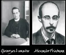
1929 : Expansion of the universe (predicted in 1922 by Alexander Friedmann and observed in 1929 by Edwin Hubble).
1960 : Gravitational spectral shift or Einstein effect (predicted in 1915 by Albert Einstein and observed in 1960 by Pound and Rebka).
1965 : Big Bang (formulated in 1927 by Georges Lemaître and confirmed in 1965 by Arno Penzias and Robert Wilson by the discovery of the cosmic microwave background representing the residual radiation of the primordial universe).
1966 : Light delay or Shapiro effect (predicted in 1964 by Irwin Shapiro and detected in 1966 and 1967 by the Haystack radar antenna at MIT).
1970 : GPS system (put into service in the 1970s-1980s by the United States Department of Defense).
1971 : Dilation of gravitational time (predicted in 1915 by Albert Einstein and confirmed in 1971 by Hafele & Keating with atomic clocks on board planes flying around the world).
1979 : Gravitational lens effect (predicted in 1936 by Albert Einstein and observed in 1979 by Dennis Walsh and his team on a double quasar).
2015 : Gravitational waves (predicted in 1916 by Albert Einstein and detected directly in 2015 by the LIGO laser, international collaboration).
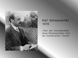
2019 : Black holes (predicted in 1916 by Karl Schwarzschid and observed in 2019 by the EHT telescope, international collaboration).
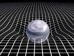
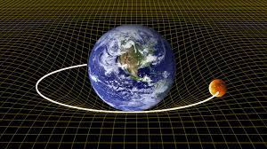
The fundamental equation of General Relativity, known as the Einstein Field Equation (EFE) or the Einstein equation of gravitational field, defines how the presence of matter and energy locally distorts the geometry of the universe (see Figure above).
John Archibald Wheeler, American specialist of General Relativity, summarizes this state as follows : "Matter tells space-time to bend and space-time tells matter how to move".
This equation can be seen as a generalization of the elasticity law of Hooke in a weakly deformed continuous medium for which the deformation of an elastic structure is proportional to the tension exerted on this structure. This equation is written in tensorial form as follows :
|
(E1) Sab = K Tab with : Sab = Rab - (1/2) gab R + Λ gab This relation links the local curvature of Space-time (tensor Sab) to the local distribution of constraints arising from matter and energy (tensor Tab) via a coupling coefficient (K). - The relationship is valid at each point of Space-time and is independent of the chosen coordinate system. In Cartesian coordinates, the units are for example m-2 for Sab and N/m2 for Tab. - The metric gab which defines the geometry of Space-time is however global because it can be influenced by distant sources (gravitational sources or energy sources). - Although the Einstein equation is a local relation, its resolution to obtain the gab metric often requires taking into account boundary conditions that can include large-scale effects, such as the Newtonian limit or the universe expansion. |
gab is the Metric tensor which is solution of Einstein Field Equation and globally defines the geometry of Space-time. The 16 gab components of this Tensor are called gravitational potentials.
Sab is the Modified Einstein tensor which measures the local curvature of the Space-time geometry. This Tensor has the remarkable property of having a zero Divergence.
This deformation of Space-time is directly related to the local presence of matter and energy via the Energy-impulse tensor Tensor Tab which encodes the properties of matter and energy.
However, this deformation can also be caused by distant sources, even in the absence of local matter and energy (i.e. when Tab = 0). In this case, the deformation is described by the Metric tensor gab which encodes the geometry of Space-time.
So, there is no gravitational force in General Relativity since this deformation of Space-time takes its place.
Tab is the Energy-impulse tensor which describes the local distribution of constraints arising from matter and energy, or any other form of non-gravitational field such as the electromagnetic field.
This Tensor depends on the pressure p and the density ρ of the physical environment that fills the space.
This Tensor is constructed so that its zero Divergence expresses the local conservation of energy and impulse.
Rab est le Ricci tensor producted by Contraction of the Curvature tensor.
R is the Scalar curvature producted by Contraction of the Ricci tensor.
a and b are the indices representing the rows and columns of all the Tensors of order 2 in the Einstein equation. These indices range from 0 to 3, each corresponding to a dimension of space-time with 0 for time.
K is the gravitational coupling coefficient : K = 8 π G c-4 = 2.0766 10-43 N-1 or kg-1.m-1.s2
This coefficient was chosen so as to verify the Poisson equation of the Newtonian gravitation as a particular case of Einstein Field Equation (see Newtonian Limit).
K represents an extraordinarily small "elasticity" of Space-time. For example, an observer located on the surface of the Sun (M_Sun = 1.99 1030 kg ; R_Sun = 6.96 108 m ; dimension n = 3) would see space-time curve according to a scalar curvature R = -K ρ c2 = -K M_Sun (3/4)(1/π) R_Sun-3 c2 = -3.0 10-24 m-2, corresponding to a curvature radius r = (n(n - 1)/|R|)1/2 = 1.0 1012 m, or approximately 2000 times the radius of the Sun.
G is the universal gravitational constant : G = 6.67408 10-11 kg-1.m3.s-2
c is the light speed in the vacuum : c = 2.99792458 108 m.s-1
Λ is the Cosmological constant of dimension m-2 and may be negative, zero or positive.
The problem of the planets motion, considered as material particles in an empty space around the sun (Schwarzschild space-time), is solved by taking Λ = 0 and Tab = 0. In cosmology, the universe model (Friedmann-Lemaitre-Robertson-Walker space-time) is determined by a priori non-zero Λ value and the universal space is considered as filled with a real gas of galaxies with density ρ and pressure p = 0 (Standard cosmological model).
This equation is sometimes presented with the "minus" sign in front of Λ and/or in front of K.
It depends on the author conventions taken for the Signature of the Metric tensor, the definition of Curvature tensor and the definition of Ricci tensor.
|
Proof : We define by (C1)(C2)(C3)(C4) the following four signs : (C1) Signature (-, +, +, +) (C2) Curvature tensor defined by Rijkl = Γijl,k + ... (C3) Ricci tensor defined by Rij = Rkikj (C4) "Einstein sign" which is the sign in front of the second member K Tab of Einstein Field Equation and corresponding to (C4) = (C2)(C3) Given the definitions (C1)(C2)(C3) and expressions : Γijk = (1/2) gil (glk,j + glj,k - gjk,l) and : R = gij Rij, Einstein Field Equation can then be put in the following form : (C2)(C3)Rab - (1/2) (C1)gab (C1)(C2)(C3)R + Λ (C1)gab = K Tab which is equivalent to : Rab - (1/2) gab R + (C1)(C2)(C3)Λ gab = (C2)(C3)K Tab Einstein Field Equation (E1) can therefore be presented in the following different forms : 1. Rab - (1/2) gab R + Λ gab = K Tab in the case (C1 = 1) and (C2, C3) = (1, 1) or (-1, -1) 2. Rab - (1/2) gab R - Λ gab = -K Tab in the case of (C1 = 1) and (C2, C3) = (1, -1) or (-1, 1) 3. Rab - (1/2) gab R - Λ gab = K Tab in the case of (C1 = -1) and (C2, C3) = (1, 1) or (-1, -1) 4. Rab - (1/2) gab R + Λ gab = -K Tab in the case of (C1 = -1) and (C2, C3) = (1, -1) or (-1, 1) Case 1 with (C2, C3) = (1, 1) corresponds to the classic sign conventions which are those of Misner, Thorne and Wheeler. |
By contracting the Einstein Field Equation by the inverse Metric tensor gab, the Scalar curvature R is related to the Energy-impulse tensor Tab by the relation :
(E2) R = -K T + 4 Λ
where T is the trace of the Energy-impulse tensor : T = gab Tab = Taa
By replacing this relation in the Einstein Field Equation (E1), we find the following equivalent equation :
|
(E3) Rab = K (Tab - (1/2) gab T) + Λ gab |
This equivalent equation may be more practical in certain cases, for example when we are interested in the weak gravitational field limit and we can replace gab by the Minkowski metric without significant loss of precision.
In the particular case where Tab = 0 (vaccum space) and Λ = 0, the Ricci tensor Rab is zero.
A solution of Einstein Field Equation of vaccum space with Λ = 0, like the Schwarzschild solution, is therefore a Metric whose Ricci tensor is identically zero. On the other hand, the Curvature tensor is not zero, except in the case of the trivial solution constituted by the Minkowski metric (flat Space-time of Restricted Relativity). cf [GOU, Relativité générale, p.119].
|
Einstein Field Equation has the following properties : Simplicity : Although General Relativity is not the only relativistic theory, it is the simplest that is devoid of internal contradictions and consistent with the experimental data. However several questions remain open : the most fundamental one is to succeed in formulating a complete and coherent theory of quantum gravitation. Postulate : Einstein Field Equation is not demonstrated on the basis of more fundamental principles. This is the whole genius of Einstein to have postulated its. Principle of equivalence (local equivalence between gravitational field and acceleration field) : Einstein Field Equation respects the Principle of equivalence. Principle of general relativity (invariance of the physical laws in any change of reference frame): Einstein Field Equation is Covariant and keep thus the same form in any change of coordinates. This is the extraordinary power of tensorial formalism : once written in tensorial form (according to Tensoriality criteria), a physical law necessarily has a form independent of the coordinates system. Conservative tensors : the members of Einstein Field Equation are both conservative (zero Divergence) to respect the principle of local conservation of impulse and energy. Zero curvature to infinity : Einstein Field Equation induces zero gravitation, and therefore zero curvature, when the coordinates tend towards the infinite (far from any attractive mass). Space-time becomes the flat Space-time of Restricted Relativity with its Minkowski metric. Newtonian gravitation : Einstein Field Equation has as their particular case the Poisson equation of the Newtonian limit. |
The 16 components of the Modified Einstein tensor Sab are function only of the gravitational potentials gab and their first and second derivatives. These components are linear with respect to the second derivatives and involve the Christoffel symbols which are function of these gab.
The resolution of these coupled differential equations of the second order is extremely difficult.
The Symmetry of the Tensors Rab, gab and Tab reduces to 10 the number of distinct equations and the 4 conditions of zero Divergence linked to the Tab Tensor reduce them to 6 independent equations.
On their side, by symmetry, only 10 of gab are distinct. In a four-space the values of 4 of them can be chosen arbitrarily which also reduces to 6 the number of functions gab to be determined.
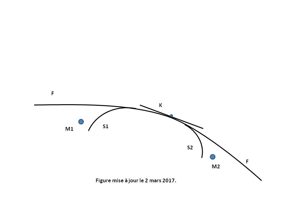
Several Relativistic Metrics are then available in General Relativity (see Figure above).
The Schwarzschild metric (S1, S2...) describes the geometry around the masses (M1, M2...), these masses can be a star, a planet or a Black hole.
The Friedmann-Lemaitre-Robertson-Walker metric (F) is used in cosmology to describe the universe evolution at large scales. It is the main tool leading to the construction of the Standard cosmological model : the Big Bang theory.
The Minkowski Metric (K) describes the geometry away from the large masses, on the asymptotically flat part of the previous metrics, according to a tangent Euclidean Space-time of Restricted Relativity.
Under the hypothesis that the gravitational field is static and centrally symmetrical (Schwarzschild metric) as the case of Sun and many stars, the gravitational potentials gab are expressed in spherical coordinates (r, θ, φ) with respect to two parameters μ and α only functions of r.
These gab allow to calculate the components of the Ricci tensor (Rab) and then, by Contraction, the Scalar curvature (R). See calculations detailed below.
In the particular case of a gravitational field in vacuum (when the Energy-impulse tensor (Tab) is zero) and a zero Cosmological constant (Λ = 0), Einstein Field Equation then is reduced to a system of two differential equations of the functions μ and α. Their integration gives the expressions μ and α. See calculation detailed below.
The Schwarzschild metric ds2 is finally completely determined as follows :
|
g00 = -(1 - r*/r) g11 = 1 / (1 - r*/r) g22 = r2 g33 = r2 sin2[θ] gij = 0 for i and j taken different between 0 and 3 |
where r* is a constant called Schwarzschild radius or gravitational radius.
In the particular case of a gravitational field created by a symmetrical central mass M, we have : r* = 2 G M c-2, producted by comparing the Schwarzschild g00 with the g00 of the Newtonian limit. In the case of Sun (with M_Sun = 1.9891 1030 kg), r* is very small and is egal to : 3.0 km
The particular values r = 0 and r = r*, which make the coefficients g00 and g11 infinite, delimit a singular region which is in practice located deep inside the mass M, which is not inconvenient for planets, ordinary stars and neutron stars for which we always have : r >> r*.
For Black holes the singularity r = r* can be eliminated by a suitable choice of the coordinate system. On the other hand, the singularity r = 0 is a singularity of the Metric tensor g which shows the limit of the Black holes description by the General Relativity and probably requires the use of a quantum theory of gravitation which does not really exist to date.
When r tends to infinity, the coefficients gab are reduced to the components of the Minkowski metric expressed in spherical coordinates. Schwarzschild space-time is thus asymptotically flat.
We finally write and solve the equations of Geodesics which describe the movement of free particles in the space considered, that is when these particles (material systems or photons) are not subjected to an external force other than gravitation in the context of General Relativity. See Geodesic of a material body and Geodesic of a photon.
|
Detailed calculation of components gab, Rab, R, Sab, α and μ [GOU, Relativité Générale, p.117] : In the case of a gravitational field with static and centrally symmetry (Schwarzschild metric), the gravitational potentials gij of the Metric tensor are the following : g00 = -e2 μ g11 = e2 α g22 = r2 g33 = (r2) sin2[θ] gij = 0 for i and j taken different between 0 and 3 where μ and α are only functions of r. The gravitational potentials gij of the inverse Metric tensor are then the following such that : gij gjk = δik where δ is the Kronecker symbol. g00 = -e-2 μ g11 = e-2 α g22 = 1/r2 g33 = (1/r2) sin-2[θ] gij = 0 for i and j taken different between 0 and 3 The Christoffel symbols Γijk are then written by the relations : Γijk = (1/2) gil (glk,j + glj,k - gjk,l) Γ001 = Γ010 = μ' Γ100 = e2 (μ - α) μ' ; Γ111 = α' ; Γ122 = -r e-2 α ; Γ133 = -r sin2[θ] e-2 α Γ212 = Γ221 = 1/r ; Γ233 = -cos[θ] sin[θ] Γ313 = Γ331 = 1/r ; Γ323 = Γ332 = 1/ tan[θ] where μ' = dμ/dr and α' = dα/dr The other Christoffel symbols are all zero. The Rij components of Ricci tensor are then written by the relations : Rij = Rkikj = Γkij,k - Γkik,j + Γkkl Γlij - Γkjl Γlik R00 = e2 (μ - α) ( μ" + (μ')2 - μ' α' + 2 μ'/r ) R11 = -μ" - (μ')2 + μ' α' + 2 α'/r R22 = e-2 α ( r (α' - μ') - 1 ) + 1 R33 = sin2[θ] R22 The other components Rij are all zero. The Scalar curvature is then written by the relation : R = gij Rij R = 2 e-2 α ( -μ" - (μ')2 + μ' α' + 2 (α' - μ')/r + (e2 α - 1)/r2 ) In the case of Λ = 0, the Modified Einstein tensor is then producted by the relation : Sab = Rab - (1/2) gab R E00 = (1/r2) e2 (μ - α) (2 r α' + e2 α - 1 ) E11 = (1/r2) (2 r μ' - e2 α + 1 ) E22 = r2 e-2 α ( μ" + (μ')2 - μ' α' + (μ'- α')/r ) E33 = sin2[θ] E22 The other components Eij are all zero. The Einstein Field Equation is then written by the relation : Sab = K Tab E00 = K T00 E11 = K T11 E22 = K T22 E33 = K T33 0 = K Tij for i and j taken different between 0 and 3 In the case Tab = 0, the Einstein Field Equation is then reduced to the 3 following equations : 2 r α' + e2 α - 1 = 0 2 r μ' - e2 α + 1 = 0 μ" + (μ')2 - μ' α' + (μ'- α')/r = 0 The first equation is integrated into : α = -(1/2) ln[ 1 - r*/r] where r* is a constant. By replacing this α value into the second equation, this one is integrated into : μ = (1/2) ln[ 1 - r*/r] + b0 where b0 is a constant. The zero of the gravitational field at infinity (so as to ensure an asymptotically flat metric with μ = 0 when r tends to infinity) requires that : b0 = 0. By replacing these α and μ values in the third equation, this one is always satisfied. We finally find : g00 = -(1 - r*/r) g11 = 1/(1 - r*/r) |


Under the hypothesis that Space-time is spatially homogeneous and isotropic (Friedmann-Lemaitre-Robertson-Walker metric), the gravitational potentials gab are expressed in spherical coordinates (r, θ, φ) with respect to two parameters k (constant) and a (function of t only).
These gab allow to calculate the components of the Ricci tensor (Rab) and then, by Contraction, the Scalar curvature (R).
By choosing a Perfect Fluid model for the Energy-impulse Tensor (Tab), its components then can be calculated as a function of the pressure p and the density ρ of the physical environment that fills the space.
The Einstein Field Equation is then reduced to a system of two differential equations of the functions a(t), ρ(t) and p(t), called Friedmann equations :
(F1) (a'/a)2 + k (c/a)2 = (1/3) ρ K c4 + (1/3) Λ c2
(F2) a"/a = -(1/6) (ρ + 3 p c-2) K c4 + (1/3) Λ c2
The system is completed by giving to cosmic fluid an equation of state as p = p(ρ). An example of a frequently used equation of state is : p(t) = w ρ(t) c2 where w is a constant that is equal to -1 (quantum vacuum), 0 (zero pressure) or 1/3 (electromagnetic radiation).
This equation of state, associated with the two equations (F1) and (F2), gives a remarkable relation linking ρ(t) and a(t) :
(Q0) ρ(t) a(t)3(1 + w) = ρ0 a03(1 + w) = constant
where ρ0 and a0 are two constants (index 0 generally corresponding to current data).
The system then reduces to a single differential equation of the function a(t) (see calculation detailed below) :
|
(Q1) (a')2 + k c2 = A a-(1 + 3 w) + B a2 (Q1a) A = (1/3) ρ0 (a0)3(1 + w) K c4 = constant (Q1b) B = (1/3) Λ c2 |
This differential equation is analytically integrated for w = -1, 0 or 1/3 (with any Λ and k), which completely determines a(t) and the metric ds2 as follows :
|
g00 = -1 g11 = a(t)2 (1 - k r2)-1 g22 = a(t)2 r2 g33 = a(t)2 r2 sin2[θ] gij = 0 for i and j taken different between 0 and 3 |
The first Friedmann equation (F1) is often presented in the condensed form :
1 + Ωk = Ω + Ωv
where :
H(t) = Hubble parameter (of dimension s-1) = a'/a that accounts for the universe expansion. See Hubble-Lemaître law
Ωk(t) = reduced curvature (dimensionless) = k (c/a)2 / H(t)2
Ω(t) = density parameter (dimensionless) = (8/3) π G ρ(t) / H(t)2
Ωv(t) = reduced Cosmological constant (dimensionless) = (1/3) Λ c2 / H(t)2
q(t) = deceleration parameter (dimensionless) = -a a"/ (a')2 = -1 - H'(t)/H(t)2
It would appear that the value to date of the deceleration parameter is negative (a" > 0), the slowing due to the matter attraction being totally compensated by the acceleration due to a hypothetical Dark energy.
The Friedmann second equation (F2) is also written in the form :
(Q2) a"/a = -F a-3(1 + w) + B
(Q2a) F = (1/2) (1 + 3 w) A
Note that the relation (Q2) is also found immediately by derivation of the relation (Q1).
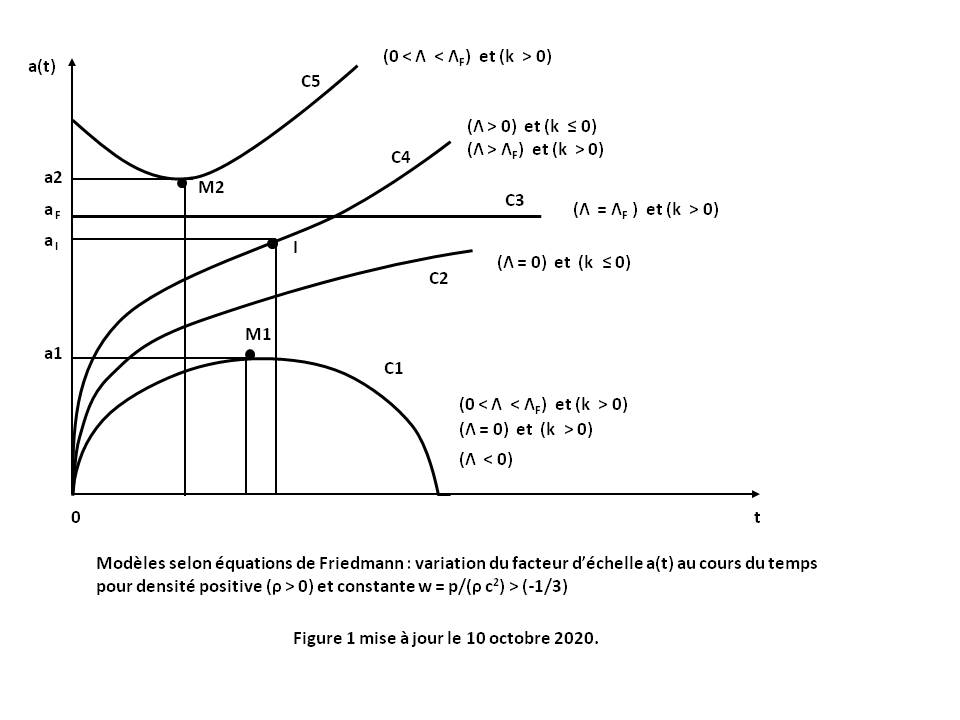
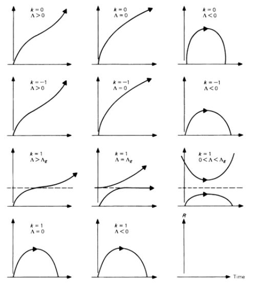
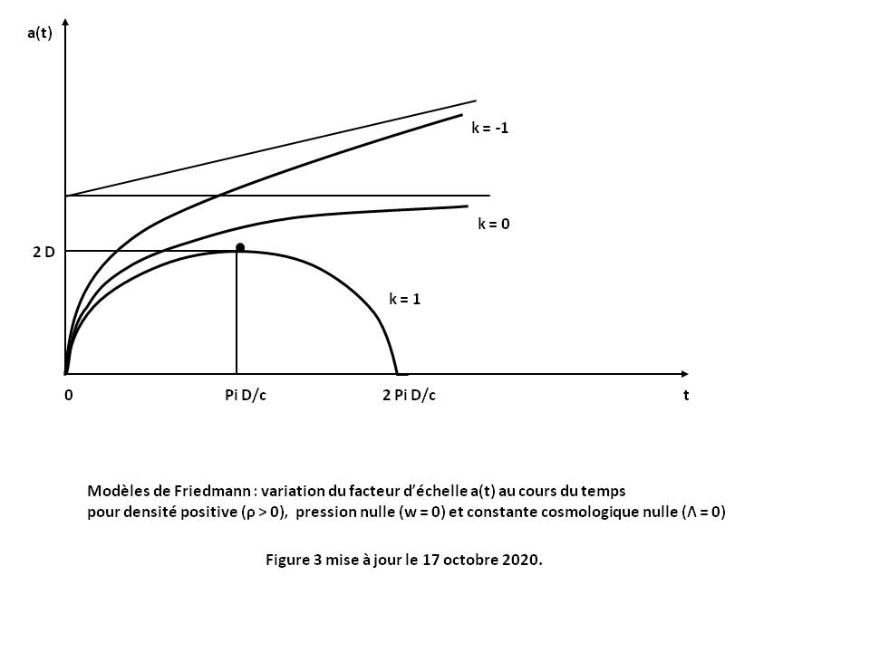
In the standard case where ρ > 0 and w > (-1/3), we then deduce from relations (Q1) and (Q2) the general shape of the curves a(t) for any Λ and k (see Figure 1 above with Proof below, or Figure 2 above cf [HAR Cosmology, table p.367] or [LUM, table p.153]).
All these curves, except two, represent Big Bang models for which a(t) tends to 0 when t tends to 0 :
- The curve C1 corresponding to case (Λ < 0), or case (Λ = 0) and (k > 0), corresponds to a closed model (decelerated expansion with a maximum point M1).
- The curve C2 corresponding to case (Λ = 0) and (k ≤ 0) correspond to an open model (decelerated expansion).
- The curve C4 corresponding to case (Λ > 0) and (k ≤ 0), or to the case (Λ > ΛF) and (k > 0) correspond to an open model with inflection point I (decelerated expansion followed by accelerated expansion). The sub-case (Λ > 0) and (k = 0) corresponds to the Standard cosmological model when the pressure is zero (w = 0).
- The curves C5, and again C1, are related to case (0 < Λ < ΛF) and (k > 0). They correspond to two possible behaviors : an open model of non-Big Bang type (accelerated expansion with a minimum point M2), and a closed model with a maximum point M1.
- The curve C3 is related to singular case (Λ = ΛF) and (k > 0). It corresponds to a static model (Einstein static universe) for which a(t) = constant. This model is unstable to density disturbances ρ with a local tendency to expansion (curve C5 after point M2) or to contraction (curve C1 before point M1).
Note that these curves represent a subset of curves listed by Harrison [HAR Classification].
ΛF is the singular Cosmological constant of Friedmann which is written (see Proof below) :
(Q6) ΛF = (1/2)(1 + 3 w) ρF K c2
(Q6a) aF = ( (1/2)(1/k)(1 + w) ρF K c2 )-1/2
For k = 1 and ρF = ρE, we get the expressions ΛE and aE of the Einstein static universe :
ΛE = (1/2)(ρE + 3 pE c-2) K c2
aE = ( (1/2)(ρE + pE c-2) K c2 )-1/2
Some particularly simple solutions for a(t) are presented below (index 0 generally corresponding to data to date).
Apart from the first two solutions, the others are almost all Big Bang models presented according to the values of parameters w, then Λ then k.
1. Einstein static universe
It is the static cosmological model with : a(t) = aE ; ρ(t) = ρE ; p(t) = pE
where aE, ρE and pE are constants.
The second Friedmann equation (F2) then becomes : Λ = ΛE
where : ΛE = (1/2)(ρE + 3 pE c-2) K c2
ΛE is the singular Cosmological constant of Einstein which characterizes a static universe.
Note that outside a vacuum (ρE = pE = 0), a static solution can exist only with a non-zero Cosmological constant.
By replacing this value of Λ in the first Friedmann equation (F1), we find :
k / aE2 = (1/2)(ρE + pE c-2) K c2
If the cosmic fluid satisfies the strict low energy condition then : ρE + pE c-2 > 0 and therefore necessarily : k > 0, so : k = 1
The curve a(t) is thus a constant (see curve C3 in Figure 1 above) :
a(t) = aE = ( (1/2)(ρE + pE c-2) K c2 )-1/2
2. De Sitter Space-time
It is the cosmological model of the vacuum (ρ = p = 0) with Λ > 0 and k = 0 (flat curvature).
The first Friedmann equation (F1) then becomes : (a'/ a) 2 = (H0)2
with H0 = B1/2 = c (Λ / 3)1/2
This equation is integrated into :
a(t) = a0 eH0 (t - t0)
where a0 and t0 are constants.
The curve a(t) is of exponential type and is not a Big Bang model.
3. Friedmann model with open curvature
It is the cosmological model without pressure (w = 0) with Λ = 0 and k = -1 (open curvature)
By replacing these values in differential equation (Q1), we find :
a'2 = A a-1 + c2
where A = A(w = 0) according to the relation (Q1a)
This equation is integrated in the form of a parametric equation :
a(t) = D (cosh[m] - 1)
t - ti = (D/c) (sinh[m] - m)
with D = (1/2) A c-2 and parameter m > 0
where a0, ρ0 > 0 and ti are constants, ti being generally set to 0 by an original choice of the coordinate t.
The term (t - ti) expressed more simply as a function of (a) in the form :
t - ti = (D/c) ( ((a/D)(2 + (a/D)))1/2 - ln[ (1 + (a/D)) + ((a/D)(2 + (a/D)))1/2 ] )
The curve a(t) is of hyperbolic type (see Figure 3 above for k = -1).
4. Friedmann model with flat curvature (or Einstein-De Sitter Space-time)
It is the cosmological model without pressure (w = 0) with Λ = 0 and k = 0 (flat curvature)
By replacing these values in differential equation (Q1), we find :
a'2 = A a-1
where A = A(w = 0) according to the relation (Q1a)
This equation is integrated into :
a(t) = ( (1/j) A1/2 (t - ti) )j
with j = 2/3
where a0, ρ0 > 0 and ti are constants, ti being generally set to 0 by an original choice of the coordinate t.
The curve a(t) is a power function (see Figure 3 above for k = 0).
5. Friedmann model with closed curvature
It is the cosmological model without pressure (w = 0) with Λ = 0 and k = 1 (closed curvature)
By replacing these values in differential equation (Q1), we find :
a'2 = A a-1 - c2
where A = A(w = 0) according to the relation (Q1a)
This equation is integrated in the form of a parametric equation :
a(t) = D (1 - cos[m])
t - ti = (D/c) (m - sin[m])
with D = (1/2) A c-2 and parameter m varying from 0 to 2 π
where a0, ρ0 > 0 and ti are constants, ti being generally set to 0 by an original choice of the coordinate t.
The term (t - ti) expressed more simply as a function of (a) in the form :
For t - ti < π (D/c) : t - ti = (D/c) ( Arccos[1 - (a/D)] - ((a/D)(2 - (a/D)))1/2 )
For t - ti > π (D/c) : t - ti = 2 π (D/c) - (expression (t - ti) of the previous case)
The curve a(t) is a cycloïde (circle point rolling on a straight line). It is symmetrical with respect to the value t - ti = π (D/c) (see Figure 3 above for k = 1).
Note that the curve goes from the "Big Bang" point (t - ti = 0) to the "Big Crunch" point (t - ti = 2 π (D/c)) through an expansion phase (a' > 0) and then a contraction phase (a' < 0).
6. Model without pressure (w = 0) with non-zero Λ
The exact solution of this model is given by [KHA Some_exact_solutions].
7. Model without pressure (w = 0) with non-zero Λ and k = 0 (flat curvature)
By replacing these values in differential equation (Q1), we find :
a'2 = A a-1 + B a2
where A = A(w = 0) and B given by relations (Q1a) and (Q1b)
This equation is integrated into :
if Λ < 0 : a(t) = (-A/B)1/3 sin2/3[ (3/2) (-B)1/2 (t - ti) ]
if Λ > 0 : a(t) = (A/B)1/3 sinh2/3[ (3/2) B1/2 (t - ti) ]
where a0, ρ0 > 0 and ti are constants, ti being generally set to 0 by an original choice of the coordinate t.
If Λ < 0, the curve a(t) is similar to the closed curve of the Friedmann model (see Figure 3 above for k = 1).
If Λ > 0, the curve a(t) have two successive expansion phases (a' > 0). The first phase is similar to the open curve of the Friedmann model (see Figure 3 above for k = -1) with deceleration (a" < 0) but leading to an inflection point I (a" = 0). The second phase is again an open curve but with acceleration (a" > 0) (see curve C4 in Figure 1 above).
8. Model for electromagnetic radiation (w = 1/3) with non-zero Λ
The exact solution of this model is given by [KHA Some_exact_solutions].
9. Model for electromagnetic radiation (w = 1/3) with Λ = 0
By replacing these values in differential equation (Q1), we find :
a'2 + k c2 = A a-2
where A = A(w = 1/3) according to the relation (Q1a)
This equation is integrated into :
For k = -1 : a(t) = E c ( (1 + (1/E)(t - ti))2 - 1 )1/2
For k = 0 : a(t) = (4 A)1/4 (t - ti)1/2
For k = 1 : a(t) = E c ( 1 - (1 - (1/E)(t - ti))2 )1/2
with E = (A)1/2 c-2
where a0, ρ0 > 0 and ti are constants, ti being generally set to 0 by an original choice of the coordinate t.
The curves a(t) are similar to the curves of the Friedmann model (see Figure 3 above for k = -1, 0 and 1).
10. Model with w > (-1/3), Λ = 0 and k = 0 (flat curvature)
By replacing these values in differential equation (Q1), we find :
a'2 = A a-(1 + 3 w)
where A = A(w) according to the relation (Q1a)
This equation is integrated into :
a(t) = ( (1/j) A1/2 (t - ti) )j
with j = (2/3) (1 + w)-1 < 1
where a0, ρ0 > 0 and ti are constants, ti being generally set to 0 by an original choice of the coordinate t.
The curve a(t) is a power function having a parabolic branch along the time axis when t tends to infinity (see Figure 3 above for k = 0).
|
Proof of the general shape of the curves a(t) according to Friedmann equations : Friedmann equations (F1) and (F2) are written in the form : (Q1) (a')2 + k c2 = A a-(1 + 3 w) + B a2 (Q2) a"/a = -F a-3(1 + w) + B (Q1a) A = (1/3) ρ0 (a0)3(1 + w) K c4 (Q1b) B = (1/3) Λ c2 (Q2a) F = (1/2) (1 + 3 w) A In the standard case where ρ > 0 and w > (-1/3), A and F are positive and we deduce that : 1. When a tends to 0, the relation (Q1) induces that the quantity (a') tends to the infinity corresponding to the primordial universe explosion (Big Bang theory). 2. When a tends to infinity, the relation (Q1) induces that : (Q3) If Λ is non-zero, B is non-zero and the quantity (a')2 behaves as the quantity (B a2) when B is positive. (Q4) If Λ is zero, the quantity (a')2 behaves like the quantity (-k c2) when k is negative and like the quantity (A a-(1 + 3 w)) when k is zero. 3. When a' and a" are zero together, this is a singular case for which Λ = ΛF. The relations (Q1) and (Q2) give the singular value ΛF as follows : (Q5) ΛF = 3 (k/m)m ( (1/n) A c-2 )-n (Q5c) n = 2/(1 + 3 w) > 0 (Q5d) m = n + 1 And the singular scale factor aF is function of ΛF as follows : (Q5a) aF = ( 3 (k/m) ΛF-1 )1/2 = ( A c-2 (m/n)(1/k) )n/2 By expressing the constant A at the singular point (aF, ρF), we finally get : (Q6) ΛF = (1/n) ρF K c2 = (1/2)(1 + 3 w) ρF K c2 (Q6a) aF = ( (1/3)(m/n)(1/k) ρF K c2 )-1/2 = ( (1/2)(1/k)(1 + w) ρF K c2 )-1/2 4. When a' is zero, the relation (Q1) is satisfied only for some following values combinaisons (Λ, k, w, A) : Λ < 0 (Λ = 0) and (k > 0) (0 < Λ < ΛF) and (k > 0) (Λ = ΛF) and (k > 0) We deduce the following results illustrated by the curves C1 to C5 in Figure 1 above : 5. If Λ is negative, B is negative : 5.1. The relation (Q2) induces that the quantity (a") is always negative. The evolution of a(t) is decelerated, with no inflection point (a" = 0). 5.2. The relation (Q1) induces that a(t) reaches a maximum (a'= 0 ; point M1 on curve C1) for which : (-B) a3(1 + w) + k c2 a(1 + 3 w) - A = 0 6. If Λ is zero, B is zero : 6.1. The relation (Q2) induces that the quantity (a") is always negative. The evolution of a(t) is decelerated, with no inflection point (a" = 0). 6.2. If k is negative, the relation (Q4) induces that a(t) tends to the straight line a(t) = c (-k)1/2 t when a tends to infinity (curve C2). 6.3. If k is zero, the relation (Q4) induces that a(t) tends to the curve a(t) = ((1/j) A1/2 t)j with j = ( (2/3) (1 + w)-1 ) when a tends to infinity (curve C2). 6.4. If k is positive, the relation (Q1) induces that and a(t) reaches a maximum (a' = 0 ; point M1 on curve C1) for which : a(1 + 3 w) = (1/k) A c-2 7. If Λ is positive, B is positive : 7.1. The relation (Q2) induces that the quantity (a") is first negative (decelerated evolution) when a tends to zero (curves C1, C2 and C4), then becomes positive (accelerated evolution) after passing through an inflection point (a" = 0 ; point I on curve C4) for which : aI 3(1 + w) = (F/B). 7.2. The relation (Q3) induces that a(t) tends to the exponential curve a(t) = exp[ B1/2 t ] when a tends to infinity (curves C4 and C5). 7.3. Singular case (curve C3) : when Λ equals ΛF, with positive k, the relation (Q1) induces that the curve a(t) has a point with horizontal tangent (a' = 0) and zero curvature (a" = 0). 7.4. When Λ is less than ΛF, with positive k, the relation (Q1) induces that the curve a(t) has two extremums (a' = 0 ; points M1 and M2). This model has two types of possible behavior : an open model (a" > 0) with a minimum point in M2 (curve C5), and a closed model (a" < 0) with a maximum point in M1 (curve C1), the respective inflection points I1 and I2 of each model being fictitious and rejected in the forbidden band (a1 < a < a2). Note that the open model of this case is not a Big Bang model. |
|
Detailed calculation of components gab, Rab, R, Sab, Tab and a(t) [GOU, Relativité Générale, p.195] : In the case of spatially homogeneous and isotropic Space-time (Friedmann-Lemaitre-Robertson-Walker metric), the gravitational potentials gij of the Metric tensor are the following : g00 = -1 g11 = a2 (1 - k r2)-1 g22 = a2 r2 g33 = a2 r2 sin2[θ] gij = 0 for i and j taken different between 0 and 3 where k is a constant (0, 1 or -1) and a is a function of t only. The gravitational potentials gij of the inverse Metric tensor are then the following such that : gij gjk = δik where δ is the Kronecker symbol. g00 = -1 g11 = a-2 (1 - k r2) g22 = a-2 (1/r2) g33 = a-2 (1/r2) sin-2[θ] gij = 0 for i and j taken different between 0 and 3 The Christoffel symbols Γijk are then written by the relations : Γijk = (1/2) gil (glk,j + glj,k - gjk,l) Γ011 = a a' (1/c)/(1 - k r2) ; Γ022 = a a' r2 (1/c) ; Γ033 = a a' r2 (1/c) sin2[θ] Γ101 = Γ110 = a' (1/c)(1/a) ; Γ111 = k r / (1 - k r2) ; Γ122 = -r (1 - k r2) ; Γ133 = -r (1 - k r2) sin2[θ] Γ202 = Γ220 = a' (1/c)(1/a) ; Γ212 = Γ221 = 1/r ; Γ233 = -cos[θ] sin[θ] Γ303 = Γ330 = a' (1/c)(1/a) ; Γ313 = Γ331 = 1/r ; Γ323 = Γ332 = 1/ tan[θ] where a' = d(a)/dt The other Christoffel symbols are all zero. The Rij components of Ricci tensor are then written by the relations : Rij = Rkikj = Γkij,k - Γkik,j + Γkkl Γlij - Γkjl Γlik R00 = -3 a" (1/a) c-2 R11 = (a a" + 2 a'2 + 2 c2 k) c-2/(1 - k r2) R22 = (a a" + 2 a'2 + 2 c2 k) (r/c)2 R33 = sin2[θ] R22 The other components Rij are all zero. The Scalar curvature is then written by the relation : R = gij Rij R = 6 c-2 ( (a"/a) + (a'/a)2 + (c/a)2 k ) with b = (a'/a)2 + k (c/a)2 The Modified Einstein tensor is then producted by the relation : Sab = Rab - (1/2) gab R + Λ gab E00 = R00 + (R/2) - Λ E11 = ( (2b + a"/a) c-2 - 3 (b + a"/a) c-2 + Λ ) a2 /(1 - k r2) E22 = E11 r2 (1 - k r2) E33 = E22 sin2[θ] The other components Eij are all zero. For a Perfect Fluid of density ρ and pressure p, the Energy-impulse Tensor of Perfect Fluid is then producted by the relation : Tij = (c2 ρ + p) ui uj + p gij The hypothesis of spatial isotropy induces that the Observer is Comoving with the fluid. The hypothesis of spatial homogeneity also induces that ρ and p are quantities function of t only. The expression of Tij are written : T00 = ρ c2 T11 = p a2 /(1 - k r2) T22 = T11 r2 (1 - k r2) T33 = T22 sin2[θ] The other components Tij are all zero. The Einstein Field Equation is then written by the relation : Sab = K Tab E00 = K T00 E11 = K T11 E22 = K T22 E33 = K T33 0 = Eij = K Tij = 0 for i and j taken different between 0 and 3 The Einstein Field Equation is then reduced to the 2 following equations : b = (1/3) ρ K c4 + (1/3) Λ c2 (1/2) b + a"/a = (1/2) Λ c2 - (1/2) p K c2 By replacing the first equation in the second one, we find Friedmann equations : (F1) (a'/a)2 + k (c/a)2 = (1/3) ρ K c4 + (1/3) Λ c2 (F2) a"/a = -(1/6) (ρ + 3 p c-2) K c4 + (1/3) Λ c2 Deriving the first equation with respect to t and replacing a" in the second one, we find the following simple relation : d(ρ)/dt = -3 (a'/a)(ρ + p c-2) In the case where the cosmic fluid has a equation of state such as : p(t) = w ρ(t) c2, this relation becomes : d(ρ)/(ρ) = -3 (1 + w)(da/a) which integrates into : ρ(t) = ρ0 (a0 / a(t))3(1 + w) where ρ0 and a0 are two constants (index 0 generally corresponding to current data). By replacing this expression of ρ(t) into the first Friedmann equation (F1), we find a differential equation that is a function of a(t) only : (Q1) (a')2 + k c2 = A a-(1 + 3 w) + B a2 (Q1a) A = (1/3) ρ0 (a0)3(1 + w) K c4 (Q1b) B = (1/3) Λ c2 |
General Relativity successfully explains three types of fundamental spectral shifts [AND Theory - Part 2] :
The Doppler-Fizeau effect which induces a spectral shift due to a speed effect of the light source with respect to the Observer.
This shift is directed indifferently towards blue or red depending on whether speed is an approach speed or distance speed but whose transverse effect is always directed towards red.
The Einstein effect which induces a spectral shift of gravitational origin due to the effect of a mass close to the source.
Radiation emitted in an intense gravitational field is observed with a shift that is always directed towards red.
The Hubble-Lemaître law which induces a cosmological spectral shift due to an effect of distance from the source.
This shift is always directed towards red.
To explain these very profound phenomena of physics, General Relativity has had to go through the successive generalizations of Space-time notion :
- Flat Space-time to interpret the Doppler-Fizeau effect.
- Curved Space-time to interpret the Einstein effect.
- Space-time with variable curvature to interpret the Hubble-Lemaître law.
Notions used in this page, listed alphabetically :
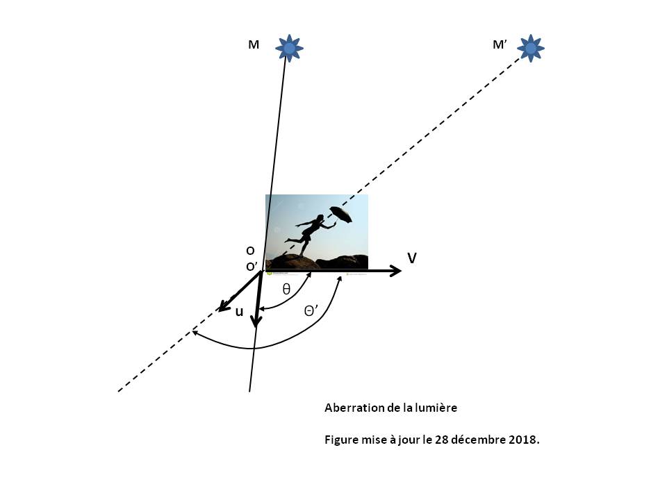
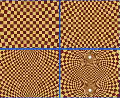
Figure 1 : Phenomenon of light aberration.
Figure 2 : Distortion of the celestial sphere. The four figures correspond to different values of the speed v of the moving observer O' (v = 0, 0.3c, 0.6c, 0.9c) [GOU, Relativité Restreinte, p.162].
The aberration of light is the difference between the incidence directions of the same light ray perceived by two Observers in relative motion.
It is not a purely relativistic effect because the aberration results from the finite time of propagation of a signal, as shown by the example of the pedestrian who walks in the rain : the rain falling vertically on the ground, the pedestrian must tilt his umbrella forward if he does not wish to be wet.
Let O be an Observer of a reference frame R and O' an Observer of a reference frame R' in uniform rectilinear translation of velocity v with respect to R.
In the case of a light source M seen by O', the light emanating from M appears to come from M' and not from M (see Figure 1 above).
u is the unit vector of the light propagation MO.
If the propagation u makes with the velocity v an angle θ in R and θ' in R', then we have the relation :
cos[θ'] = (cos[θ] - v/c) / (1 - cos[θ] v/c)
Using the relation : tan2[θ/2] = (1 - cos[θ])/(1 + cos[θ]), we have the equivalent relation :
|
tan[θ'/2] = ( (1 + v/c)/( 1 - v/c) )1/2 tan[θ/2] |
So we always have : θ' > θ, as if the light received by the mobile Observer concentrated on its movement direction.
- When the propagation u is parallel to the velocity v in the reference frame R (θ = 0 or π), then the formula reduces to : cos[θ'] = 1 or -1, which induces : θ' = 0 or π, and there is no aberration effect.
- When u is perpendicular to v in the reference frame R (θ = π/2), then the formula reduces to : cos[θ'] = -v/c, which induces : θ' > π/2 (and the pedestrian must tilt his umbrella forward).
For a terrestrial Observer O' (v = 30 km.s-1), the Image of a star located at the north pole of the ecliptic (θ = π/2) thus describes in a year a circle of radius 20'' around this pole. Not to be confused with the parallax which is the view angle of a star when Earth travels its orbit and which is at most 0.77'' for the nearest star (Proxima Centauri) [GOU, Relativité Restreinte, p. 162].
- When v is small compared to c, there is no aberration effect (θ' = θ).
The aberration phenomenon is visualized very well by considering a uniform grid on the celestial sphere of the Observer O (see Figure 2 above). The Observer O' sees directions appearing out of the field for the Observer O, until seeing the two celestial poles at the same time.
Relativistic aberration of light was demonstrated directly by Daniel Giovannini's team at the University of Glasgow, in a terrestrial laboratory.
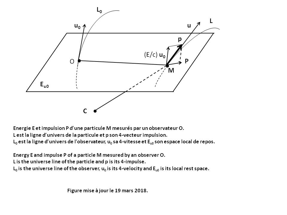
The angular momentum vector σC of a particle M relative to a given point C and mesured by an Observer O in his Local reference frame at time τ is given by the following relation (see Figure above) [GOU, Relativité Restreinte, p.322] :
|
σC = CM xu0 P |
P is the Impulse vector of the particle.
u0 and Eu0 are the Quadri-velocity of the Observer and his Local rest space Eu0.
"xu0" is the Cross product operator between two any vectors of Eu0, what is written : CM xu0 P = Ε(u0, CM, P, .)
where :
Ε is the Levi-Civita tensor
Ε(u0, CM, P, .) is the vector representing the Linear form Ε(u0, CM, P, z) for the Scalar product g.
σC belongs to Eu0 and its components are of dimension kg.m2.s-1
See Symmetry and antisymmetry.
Let [A] be the transition matrix from base {ei} to base {e'k} such that : e'k = Aik ei, and [B] = [A-1] the inverse transition matrix such that : ei = Bik e'k
For any tensor T of order 2, using the multilinearity of T and the properties of Covariance and contravariance, the components of the tensor T' are given by the following laws :
T'ij = Aki Alj Tkl
T' ij = Bik Bjl Tkl
T' ij = Bik Alj Tkl
The base change transforms the tensor T into a tensor T' whose components are linear combinations of the components of the origin tensor.
For any tensor T p times contravariant and q times covariant, the general transformation law is as follows [GOU, Relativité Restreinte, p. 476] :
|
T' i1... ip j1... jq = (Bi1 k1)... (Bip kp) (Al1 j1)... (Alq jq) T k1... kp l1... lq |

Definition :
The Big Bang is a word with a double meaning :
- Event marking the beginning of the expansion of the universe, without this prejudging the existence of an "initial moment" or a beginning to its history.
- Standard cosmological model describing the evolution of the universe from an infinitely dense and incredibly hot state (1013 C) to the present.
The Big Bang, wrongly called a "primordial explosion", is in fact a "primordial expansion" such that the scale factor a(t) tends towards 0 when t tends towards 0. There is no ejection of matter from of a place in the universe but expansion of space reduced to a point, which takes with it all the objects of the universe.
The Big Bang was formulated in 1927 by Georges Lemaître and confirmed in 1965 by Arno Penzias and Robert Wilson by the discovery of the cosmic microwave background representing the residual radiation of the primordial universe.
Simplified chronology (see [The secrets of space] and http://scphysiques.free.fr/2nde/documents/Histoire_atome/bigbang.html ) :
- Between 0 and 10-43 seconds after the Big Bang, corresponding to "Planck time", a sort of incompressible temporal quantum according to quantum physics, our physics is silent but scientists believe that at the end of this period gravity separated itself from the other forces of nature (strong nuclear force, weak nuclear force and electromagnetic force).
- Between 10-43 and 10-6 seconds after the Big Bang, scientists describe the evolution of the universe based on hypotheses. The Big Bang can only be described according to known physics equations from 10-6 seconds.
- Around 10-32 seconds after the Big Bang, one hypothesis is that the universe was a "soup" of elementary particles and anti-particles. Some still exist today in the form of quarks, anti-quarks and bosons like gluons. Others no longer exist, such as gravitons (hypothetical particles that transmit gravity) and Higgs bosons which transmit mass to other particles.
- 300 000 years after the Big Bang, when the temperature dropped to around 2700 C, the first hydrogen and helium atoms were formed. The electrons then being linked to the atoms, matter and radiation become decoupled. Photons can then travel through the universe in the form of radiation. They reach Earth not as visible light but as low-energy photons from the cosmic microwave background.
- 200 million years after the Big Bang, the first stars appeared, made almost exclusively of hydrogen and helium. During their lives and deaths, these early stars create new chemical elements from nuclear fusion in the hot cores of these stars, such as carbon, oxygen, silicon, and iron. These chemical elements are scattered throughout space and other galaxies.
- The second and third generations of stars form later in this enriched interstellar medium. They create even more chemical elements sent back into the interstellar medium via solar winds and supernova explosions.
- The Universe history then continues with the creation of our Sun, the Earth and life on Earth. Note that the Earth will never receive visible light before the combustion of the first stars.
- Today the universe is extremely sparse (a few atoms per cubic meter) and cold (-271 C).
A black hole is a celestial object so compact that the intensity of its gravitational field prevents any form of matter or radiation from escaping from it.
This phenomena was predicted in 1916 by Karl Schwarzschild.
The first direct image of a black hole was published in 2019 by the Event Horizon Telescope (EHT), an international collaboration.
The ordinary black hole (called "stellar black hole")) is formed following the succession of several events :
- Collapse (implosion) of a massive star at the end of its life, under the effect of gravity which is no longer counterbalanced by nuclear fusion reactions.
- Explosion where the outer layers of the star are expelled into space in an intense and luminous form (supernova).
- Gravitational collapse of the core residue after the explosion if the latter has sufficient mass, which leads to the formation of a black hole.
The static black hole (without rotation) is described by the Schwarzschild Metric.
The rotating black hole not electrically charged is described by the Kerr Metric which generalizes the Schwarzschild Metric.
The rotating electrically charged black hole is described by the Kerr-Newman Metric which also generalizes the Schwarzschild Metric.
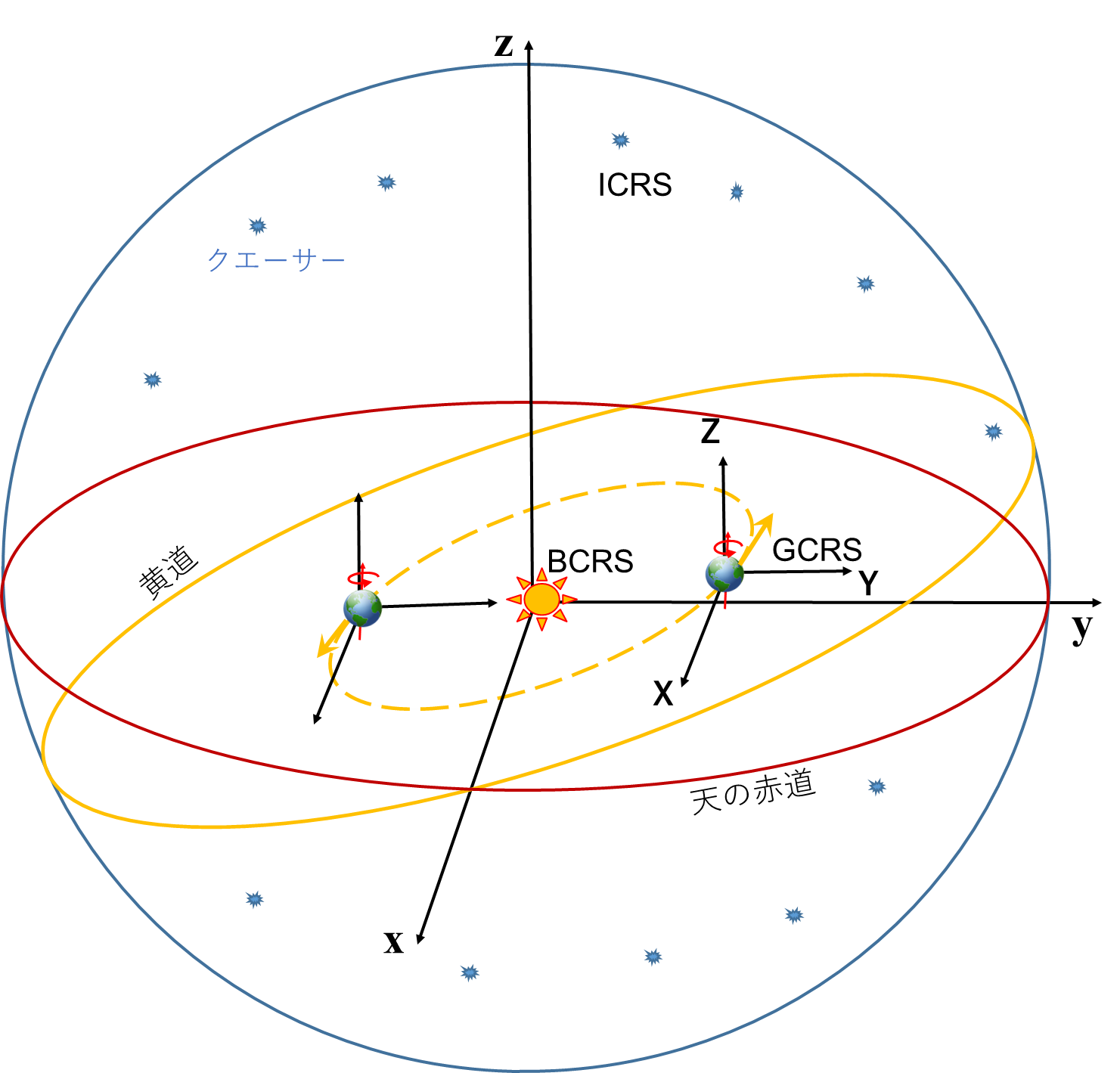
In geophysics the celestial reference frame is a reference system whose orthogonal axes (x, y, z) are defined using reference points sufficiently distant to appear fixed on the celestial sphere. These distant objects are extragalactic radio-sources.
Several celestial reference frames exist (cf [ZIEGLER, Modélisation, p.24]) :
The International Celestial Reference System (ICRS), adopted in 1997 by the International Astronomical Union (IAU), has its origin in the barycenter of the Solar System in accordance with General Relativity. Its pole (z-axis) is currently approximately in the direction of the Polar Star (Polaris). The origin of straight ascents (x-axis) is in the direction defined from quasar 3C 273, in the direction of the vernal point which is the position of the Sun seen from Earth at the spring equinox. The third axis (y-axis) is orthogonal to the first two and oriented so that the three axes form a direct direction trihedron.
The Barycentric Celestial Reference System (BCRS), defined in 2000 and 2006 by the IAU, merges with the ICRS in terms of orientation and origin but also defines a Relativistic metric for the coordinate system. The proper time of BCRS is called Barycentric Coordinate-Time (BCT).
The Geocentric Celestial Reference System (GCRS) differs from the BCRS in its origin, which is the mass center of Earth. The proper time of GCRS is called Geocentric Coordinate-Time (GCT).
These three reference frames have in common a conventional and theoretically invariable orientation (non-rotating with respect to the stars). They do not follow the rotation of the Earth over time as the terrestrial reference frames would do.
Among the terrestrial reference frames, the current standard is the International Terrestrial Reference System (ITRS) which is in daytime co-rotation with the Earth and originates from its center of mass. The proper time of ITRS is called Terrestrial Time (TT).
For a vector space of dimension n having for basis vectors the set (e1, e2... en), the Christoffel symbols Γijk (called "of second kind") represent the basic vectors evolution as a function of their partial derivative. Using the Convention of partial derivative and the Convention of summation, this is written :
|
ej,k = Γijk ei |
Warning : Although possessing three indexes, the Christoffel symbols of second kind are not mixed Tensors of order 3 because they do not satisfy the Tensoriality criteria. For example, the index lowering : Γjik = glj Γlik is not possible, which is false considering that : glj Γlik = Γijk
In contrast, they appear abundantly in expressions which represent Tensors (for example : Covariant derivative, Divergence, Ricci Tensor).
Γijk can be written as a function of basis vectors of Dual space :
|
Γijk = ei.ej,k Proof : ei.ej,k = ei.(Γijk ei) = Γijk δii = Γijk where δ is the Kronecker symbol. |
Note that there is another Christoffel symbols Γijk (called "of first kind") defined by the relation :
|
Γijk = glj Γlik = Γkji Γijk = gil Γjlk = Γikj Warning : For Γijk, there is a variant with the following different definition (by reversing the order of the indexes i and j) : Γijk = gli Γljk = Γikj |
Γijk and Γijk can be written as a function of the components gij of the Metric tensor :
|
Γijk = (1/2) (gij,k + gjk,i - gik,j) Γijk = (1/2) gil (glk,j + glj,k - gjk,l) Proof : By deriving gij = ei.ej with respect to xk, we find : gij,k = (ei,k).ej + ei.(ej,k) = (Γlik el).ej + ei.(Γljk el) This is written : gij,k = Γlik glj + Γljk gil A circular permutation of the three indexes i, j, k then gives the following two equalities : gki,j = Γlkj gli + Γlij gkl gjk,i = Γlji glk + Γlki gjl We then find by linear combination : (D) gij,k + gki,j - gjk,i = 2 Γlkj gil By reversing the roles of i and j in relation (D), we find : gij,k + gkj,i - gik,j = 2 Γlki gjl Given the Symmetries of Γlki and gjl, we finally find : Γijk = glj Γlik = (1/2) (gij,k + gjk,i - gik,j) By multiplying the two members of relation (D) by gmi and using the relation gmi gil = δml, we find : Γmkj = (1/2) gmi (gij,k + gki,j - gjk,i) By renaming the indexes (i to l and m to i), we finally find : Γijk = (1/2) gil (glk,j + glj,k - gjk,l) |
Properties :
Γijk is Symmetric with respect to the two extreme indexes : Γijk = Γkji
Γijk is Symmetric with respect to the lower index : Γijk = Γikj
Derivative of metric : gij,k = Γijk + Γjik
Index contraction (cf [GOU, Relativité restreinte, p.506]) : Γiji = (-g)-1/2 ((-g)1/2),j
with : g = Determinant of the matrix gij associated with Metric Tensor g
The Christoffel symbols are all zero only in the particular case of Restricted Relativity (Minkowski metric) with Cartesian coordinates, for which the components gij are all constant.
Two material objects are said to be comoving when they are fixed relative to each other in a given reference frame. They then share the same spatial movement, whether in Restricted Relativity (where they have the same speed in an Inertial frame) or in General Relativity (where they follow parallel Geodesics in curved Space-time).
The composition law of speeds in Restricted Relativity is as follows :
Let three orthonormal reference frames R, R' and R" initially coincident at t = t' = t" = 0, with their respective axes parallel.
R' performs a uniform rectilinear translation at constant velocity v relative to R (measured in R), followed by R" at constant velocity u relative to R' (measured in R'), these velocities may or may not be collinear.
The composite velocity w of an object stationary in R" relative to R (measured in R) is then written :
1. Case where the velocities u and v are collinear and parallel to the x-axis (see demonstration in Lorentz-Poincaré Transformation) :
(C16) w = (v + u) / (1 + v u / c2)
which can also be written as :
(1 - w/c) = (1 - v/c)(1 - u/c)
This multiplicative form shows that the composite speed w can never exceed the speed of light and that, at high speeds, the composition law is no longer additive but multiplicative in terms of relative deviations from c.
2. Case where the velocities u and v are collinear, without being aligned with a particular axis :
Relation (C16) of case 1 above does not contain any explicit reference to the spatial coordinates x, y and z.
Consequently, relation (C16) is independent of the spatial orientation of the velocities u and v, provided that they are collinear.
This case therefore comes down to case no. 1 above.
3. Case where the velocities u and v are not collinear :
The expression of the composite velocity w is complex and depends on the order of application of the transformations (first v in the reference frame R, then u in the reference frame R').
Furthermore, the vector expression of w can present differences according to the authors, linked to the definition of velocities u, v and w, as well as to the reference frame of each of these velocities. In the scientific literature, the standard situation is often the following :
* velocity v of R' / R, measured in R
* velocity u of R" / R', measured in R'
* composite velocity w of R" / R, measured in R
This convention allows a direct and consistent application of the velocity composition formula in Restricted Relativity, while avoiding potential ambiguities in the interpretation of the results [GOU, Relativité Restreinte, p.142].
In order to lighten the expressions of the derivatives of functions dependent on n variables f(x1, x2... xn), we denote the partial derivatives in the following forms :
|
f,i = di(f) = d(f)/d(xi) f,i,j = dij(f) = d2(f)/(dxi dxj) grad(f) = gradient of any function f. In any Natural base, its coordinates are [GOU, Relativité Restreinte, p.500] : ( grad(f) )i = d(f)/d(xi) div(v) = divergence of any vector v. In any Natural base, it is given [GOU, Relativité Restreinte, p.507] : div(v) = (-g)-1/2 d( (-g)1/2 vi )/d(xi) Δ(f) = Laplacian of any function f = div(grad(f)) Δ(v) = Laplacian of any vector v = grad(div(v)) - rot(rot(v)). Its coordinates are : (Δ(v))i = Δ(vi) ◊() = Alembertian of any function f or vector V. It is given [GOU, Relativité Restreinte, p.594] : ◊() = gij (d/dxi) (d/dxj) In a Inertial reference frame : ◊() = - c-2 d2()/dt2 + d2()/dx2 +d2()/dy2 +d2()/dz2 curl(v) = curl operator of any vector v. In any Natural and Orthonormal base, its coordinates are [GOU, Relativité Restreinte, p.510] : ( curl(v) )i = εijk d(vk)/d(xj) with : g = Determinant of the matrix gij associated with Metric Tensor g gij = inverse components of the Metric tensor εijk = Levi-Civita symbol Properties : div[curl()] = 0 curl[grad()] = 0 Δ(v) = grad[div(v)] - curl[curl(v)] ◊() is invariant by Lorentz-Poincaré Transformation. |
|
Proof of invariance of Alembertian operator by Lorentz-Poincaré Transformation : Alembertian operator ◊ in an Inertial reference frame can be written : ◊ = d2/dx2 + d2/dy2 + d2/dz2 - c-2 d2/dt2 = C1 C2 + d2/dy2 + d2/dz2 C1 = d/dx - c-1 d/dt C2 = d/dx + c-1 d/dt Let the simplified case where the x' axis of the reference frame R' is parallel to the x axis of the reference frame R (see Lorentz-Poincaré Transformation). The relations (L1) and (L2) give by partial derivation : d/dx = (d/dx')(dx'/dx) + (d/dt')(dt'/dx) = γ ( (d/dx') - (d/dt') β c-1 ) d/dt = (d/dx')(dx'/dt) + (d/dt')(dt'/dt) = γ ( (d/dt') - (d/dx') β c ) d2/dy2 = d2/dy'2 d2/dz2 = d2/dz'2 Replacing of these expressions in C1 and C2 gives : C1 = γ (d/dx' - c-1 d/dt') (1 + β) C2 = γ (d/dx' + c-1 d/dt') (1 - β) Given the expression of γ (relation (L3)), we then find the following result : ◊ = (d/dx' - c-1 d/dt')(d/dx' + c-1 d/dt') + d2/dy'2 + d2/dz'2 = C1' C2' + d2/dy'2 + d2/dz'2 = ◊' The identity : ◊ = ◊' shows that Alembertian operator is invariant by any change of Inertial reference frame. |
For a vector space of dimension n having as its basis vectors the set (e1, e2... en), any vector x of this space can be written : x = x1 e1 + x2 e2 + ... + xn en = ∑k=1, n[xk ek]
In order to simplify this writing we use a notation convention consisting in deleting the symbol "Sum" which is written in condensed form :
|
x = xk ek where the index k (called mute index) always varies from 1 to n. |
The summation is done on the index provided that they are repeated respectively up and down in the same monomial term.
When the prime symbol is used to distinguish two distinct bases of the same vector space, we can further simplify the notation by placing the prime symbol on the index rather than on the vector: x = x'k e'k = xk' ek'
Some terms in a sum may have several indexes. For example, in the sum akm bm, the summation is done on the index m. The index k (called free index) characterizes a particular term.
For example the equation ck = akm bm for n = 3 represents the system of equations :
c1 = a11 b1 + a12 b2 + a13 b3
c2 = a21 b1 + a22 b2 + a23 b3
c3 = a31 b1 + a32 b2 + a33 b3
There is no summation here on the index k which is found alone in the same monomial term.
When the monomial term has several mute index the summation takes place simultaneously on all these indexes. For example, akm bm ck for n = 4 represents a sum of 16 terms :
akm bm ck = a11 b1 c1 + a12 b2 c1 + a13 b3 c1 + a14 b4 c1 + ... + a21 b1 c2 + ... + a44 b4 c4
The convention of summation also applies to Partial derivative (example : gil,l) and to Covariant derivative (example : Fkl;l), although the derivative symbol is not a covariant index [DENIS, Cours, p.25].
For the Covariant derivative, the contraction of the index of a tensor by the derivation index is indeed legitimate due to the tensorial nature of the Covariant derivative and the linearity property of tensors.
Cosmic time is the Proper time of an Observer at rest in a cosmological universe which is, with the exception of local irregularities, homogeneous and isotropic.
This is the time used in the Friedmann-Lema tre-Robertson-Walker equations.
It is also the Proper time common to all galaxies to the extent that they are all Comoving with the Observer [Andrillat, Theory Part 2].
The history of Cosmological constant Λ is particularly eventful :
- In 1915 Einstein publishes his Equation of General Relativity, without a cosmological constant Λ.
- In 1917 Einstein adds the parameter Λ to his Equation when he realizes that his theory implies a dynamic Universe for which space is function of time. He then gives this constant a very particular value to force his Universe model to remain static and eternal (Einstein static universe), which he will later call "the greatest stupidity of his life".
- In 1922 the Russian physicist Alexander Friedmann mathematically shows that Einstein Field Equation (whatever Λ) remains valid in a dynamic Universe.
- In 1927 the Belgian astrophysicist Georges Lemaître shows that the Universe is in expansion by combining General Relativity with some astronomical observations, those of Hubble in particular.
- In 1931 Einstein finally accepts the theory of an expanding Universe and proposed, in 1932 with the Dutch physicist and astronomer Willem de Sitter, a model of a continuously expanding Universe with zero cosmological constant (Einstein-De Sitter Space-time).
- In 1998 two teams of astrophysicists led, one by Saul Perlmutter, the other by Brian Schmidt and Adam Riess, carrie out measurements on distant supernovae and show that the speed of galaxies recession in relation to the Milky Way increases over time. The Universe is in accelerated expansion, which requires having a strictly positive Λ. The Universe would contain a mysterious Dark energy producing a repulsive force that counterbalances the gravitational braking produced by the matter contained in the Universe (see Standard cosmological model).
For this work, Perlmutter (American), Schmidt (American-Australian) and Riess (American) jointly received the Nobel Prize in physics in 2011.
- In 2015 the value of the cosmological constant is estimated at Λ = 1,11 10-52 m-2
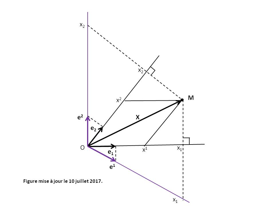
The notions of covariant and contravariant vectors apply to non-orthonormal referentials, which explains why they are not addressed in secondary or even higher mathematics courses. For Orthonormal base there is no difference between covariant and contravariant components.
For a vector space E of dimension n having for basis vectors the set (e1, e2... en), we call (see Figure above) :
|
contravariant components of a vector x the numbers xi such that : x = xi ei Covariant components of a vector x the numbers xj such that : xj = x.ej. |
The contravariant components are noted with higher indexes.
The covariant components are noted with lower indexes.
The contravariant (respectively covariant) name derives from the fact that these components are transformed by base change in an inverse (respectively identical) manner to that of the basic vectors.
When the indexes vary from 0 to 3, Greek letters (such as α or μ) are often used rather than Latin letters (such as i or j).
We have the following relations :
|
xj = gij xi xi = gij xj x.y = gij xi yj = gij xi yi |
where the coefficients gij are the components of the Metric tensor.
|
Note that the covariant components xj can also be defined in a Dual base in the form : x = xj ej where the ej are the basis vectors of the Dual vector space E* (see Figure above). |
|
Proof of the contravariant (respectively covariant) name : Consider the base change from base {ei} = (e1, e2... en) to base {e'k} = (e'1, e'2... e'n). Let [A] be the transition matrix from base {ei} to base {e'k}. The elements of [A] are Aik such that : e'k = Aik ei The higher index is the line index of the matrix. The lower index is the column index of the matrix. Let [B] = [A-1] be the inverse transition matrix from base {e'k} to base {ei} such that : ei = Bik e'k For the contravariant components, we have : x = xi ei x = x' k e'k = x' k (Aik ei) = (Aik x' k) ei Hence : xi = Aik x' k And so : x' i = Bik xk The contravariant components are transformed by base change in an inverse manner to that of the basic vectors (with inverse transition matrix [B]). For the covariant components, we have : xj = x.ej x'k = x.e'k = x.(Ajk ej) = Ajk (x.ej) = Ajk xj The contravariant components are transformed by base change in an identical manner to that of the basic vectors (with transition matrix [A]). |

The general covariance of a physical law has nothing to do with the Covariance of the tensor components. The word "covariance" does not refer to the covariant index of a Tensor but only indicates a writing of the physical law which remains form-invariant under any coordinates transformation (invariance by diffeomorphism) [AMI Initiation_aux_Tenseurs, p.18].
When the physical law can be written in the tensorial form : T = 0, or what amounts to the same : P = Q with T = P - Q (T, P and Q being Tensors of the same type), any change of reference frame transforms this equation into the tensorial form : T' = 0, which does not change the form of the physical law.
|
Proof : Let us take the example of a physical law written in the form of the tensor equation : T = 0, T being a mixed tensor of order 2. Let [A] be the transition matrix of base {ei} to base {e'k} and [B] = [A-1] the inverse transition matrix. Base change transforms the components Tij = 0 of this equation into : T' ij = Bik Alj Tkl = 0 which does not change the form of the physical law. |
Example of Newton's law : F = m γ
The covariant expression of this law is then in contravariant components [AMI Initiation_aux_Tenseurs, p.18] :
Fi = m vi;t
with : vi = dxi/dt
The term vi;t is the Covariant Derivative of the velocity dxi/dt with respect to time t, which is :
vi;t = vi;k (dxk/dt) = vi,k (dxk/dt) + Γijk vj vk = dvi/dt + Γijk vj vk
where Γijk are the Christoffel symbols.
If moreover the force F derives from a potential in the form : F = -grad(Φ), then F can be written in contravariant components : Fi = gij Fj = -gij dΦ/dxj
where gij are the inverse components of the Metric tensor.
Newton's law is then written in the following tensorial form :
|
gij dΦ/dxj + m ( d2xi/dt2 + Γijk (dxj/dt) (dxk/dt) ) = 0 |
In this tensorial form, Newton's law will remain form-invariant under any coordinates transformation (spherical coordinates for example).
Another example : Maxwell equations.
The covariant derivative is the general expression of the derivative which remains form-invariant under any coordinates transformation. It helps to make the physical laws Covariant.
According to the general procedure stated by Einstein [BARRAU, Relativité générale, p.64], "we find the correct physical laws by replacing the usual derivatives by covariant derivatives".
Using the Convention of partial derivative and the Convention of summation, for each Tensor U of order (n), its covariant derivative is the tensor of order (n + 1) of the following components (denoted u ;l or Dl u) :
|
For scalar : u;l = u,l For contravariant vector : um;l = um,l + ur Γmrl For covariant vector : ui;l = ui,l - ur Γril For contravariant Tensor of order 2 : Umn;l = Umn,l + (Urn Γmrl + Urm Γnrl) For covariant Tensor of order 2 : Uij;l = Uij,l - (Urj Γril + Uri Γrjl) For mixed Tensor of order 2 : Umi;l = Umi,l + Uri Γmrl - Umr Γril ... For mixed Tensor of order 5 : Umnijk;l = Umnijk,l + (Urnijk Γmrl + Urmijk Γnrl) - (Umnrjk Γril + Umnrik Γrjl + Umnrij Γrkl) |
where Γijk are the Christoffel symbols.
The cross product of any two vectors v and w in an n-dimensional vector space is the Tensor T = v x w of order n-2 which components are as follows :
|
Ti1i2... in-2 = εi1i2... in-2jk vj wk |
where εi...jk is the Levi-Civita symbol
Vector space E of dimension 3 :
The cross product is a vector T of components :
In covariant components : Ti = εijk vj wk
In contravariant components : Ti = gil Tl = gil εljk vj wk
gij are the inverse components of the Metric tensor.
Vector space E of dimension 4 [GOU, Relativité Restreinte, p.87] :
In the Local rest space of the observateur Eu (see Figure in Local reference frame), the cross product (noted xu) between any two vectors v and w of Eu is a vector which is written : v xu w = Ε(u, v, w, .)
where :
Ε is the Levi-Civita tensor
Ε(u, v, w, .) is the vector representing the Linear form Ε(u, v, w, z) for the Scalar product g.
The word "curvature" has several meanings in Relativity :
|
- Curvature tensor (or Riemann-Christoffel tensor) of Space-time, which is a Tensor of order 4. - Ricci Tensor of Space-time, which is a Tensor of order 2. - Scalar curvature R of Space-time, which is a Tensor of order 0 (scalar). - Curvature k* of the spatial hypersurfaces (related to the spatial curvature parameter k), which is a scalar used in the Friedmann-Lemaitre-Robertson-Walker Metric. Not to be confused with the Scalar curvature R of Space-time. - Curvature a of the Universe line of a material particle. |
The first three curvatures depend only on the gravitational potentials gab and their first and second derivatives with respect to the coordinates. In Minkowski Metric, they are all zero and correspond to the flat Space-time of Restricted Relativity.
Figures above from left to right : Georg Friedrich Bernhard Riemann and Elwin Bruno Christoffel
The curvature tensor is a Tensor of order 4. It is the most complete measure of the local deformation of a curved Space-time. It has 44 = 256 components.
According to the Classic Sign Conventions (MTW) and using the Convention of partial derivative, its componants have as expression :
|
Rijkl = Γijl,k - Γijk,l + Γimk Γmjl - Γiml Γmjk |
where Γijk are the Christoffel symbols.
The number of independent components of the curvature tensor is equal to 20 (instead of 256).
In Cartesian coordinates, all the components are of dimension m-2
The Space-time is called "flat" when the curvature tensor is zero.
Warning : Unlike classic MTW sign conventions, some authors define the Tensor of curvature by the opposite of the Tensor of curvature above [GOU, Relativité générale, p.110].
Properties :
Rijkl is Antisymmetric with respect to the two last indexes : Rijkl = -Rijlk
Rijkl is Antisymmetric with respect to the two first and last indexes : Rijkl = -Rjikl = -Rijlk
Rijkl is Symmetric with respect to the two pairs of extreme indexes : Rijkl = Rklij = Rjilk
where : Rijkl = gim Rmjkl
First identity of Bianchi : Rijkl + Riklj + Riljk = 0, also written : Ri[jkl]
Second identity of Bianchi : Rijkl;m + Rijlm;k + Rijmk;l = 0, also written : Rij[kl;m]
Identity of Ricci :
For any Contravariant vector v we have : Rijkl vj = vi;l;k - vi;k;l
Curvature tensor thus measures the non-commutativity of double Covariant derivatives [GOU, Relativité générale, p.109].
Another identity [SEN, Relativité générale, p.62] :
For any doubly Contravariant Tensor T we have : Rijkl Tjm + Rmjkl Tij = Tim;l;k - Tim;k;l
Dark energy is an hypothetical global repulsive force uniformly filling the entire universe, which tends to accelerate the universe expansion (therefore requiring : Λ > 0).
See Standard cosmological model.
Dark matter is a hypothetical material providing extra gravity that galaxies need to avoid breaking apart during their rotation.
See Standard cosmological model.
See simple explanation in Time relativity, simple definition in Time, rigorous definition in Lorentz factor and practical application in GPS.
|
Demonstration of the relation : (t'B - t'A) > (tB - tA) in Restricted Relativity [PER] : Let two events A and B occur in the frame of reference R at different locations (xA and xB) and at different times (tA and tB). For an Observer of the referential frame R' in uniform rectilinear translation at the speed v with respect to R, the events occur at instants t'A and t'B given by the Lorentz-Poincaré transformation : Δt' = t'B - t'A = γ (tB - B xB) - γ (tA - B xA) = γ Δt ( 1 - B (Δx/Δt) ) = γ Δt (1 - (v/c)T) with : Δt = tB - tA T = Δx/(c Δt) Δx = xB - xA Three cases are then possible : 1. Events occurring at the same place in R ( Δx = 0 ) : Δt' = γ Δt > Δt since : γ > 1 2. Space-type separation ( |T| > 1 ) : Δt' can be smaller than Δt, or even of opposite sign 3. Time-type separation ( |T| < 1 ) : Δt' can be smaller than Δt. In cases 2 and 3, the modification of durations (dilation or contraction) depends on the specific relationship between the relative velocity (v/c) and the spatio-temporal separation (T) of the events. In conclusion, durations dilation is not universal. It is always true in Restricted Relativity for a pair of events occurring at the same location, but might not apply for arbitrary pairs of events separated by a time-like interval. |
Gravitational time dilation is a phenomenon of general relativity that states that time passes more slowly in the presence of a gravitational field.
Thus, a clock located far from a large mass (such as a planet or a star) will indicate a longer time compared to a clock located near a large mass (in a stronger gravitational field).
This phenomenon was predicted in 1915 by Albert Einstein.
In 1971, J.C. Hafele & R.E. Keating conducted an experiment that consisted of embarking four cesium atomic clocks on airliners for a round-the-world trip (with stopovers) and comparing the time measured by these clocks with identical clocks that remained on the ground on the return trip.
This is a realization of the famous twin paradox bis.
The experiment fully confirmed the Einstein Effect of gravitational time dilation (general relativity) as well as the dilation of durations for moving bodies (special relativity) [GOU, General Relativity, pp 222, 269].
If ei are the basic vectors of Space-time, the base {ei} is called [GOU, Relativité Générale, p.21] :
|
direct when : Ε(e0, e1, e2, e3) > 0 and indirect when : Ε(e0, e1, e2, e3) < 0 |
where Ε is the Levi-Civita tensor.
The divergence of a vectors field accounts for the infinitesimal variation of the volume (or electric charge) around a point. The divergence of a Tensor generalizes this notion.
The divergence of a Tensor U of order (n) is the tensor Div(U) of order (n - 1) producted by contracting one of the index of the Covariant derivative with the derivation index.
For a twice contravariant Tensor, there are two possible divergences : right divergence (component Uij ;j) and left divergence (component Uij ;i). The divergences are equal only if the tensor is Symmetric or Antisymmetric.
Example : Modified Einstein tensor Sab has zero divergence (Sab;a = 0).
Properties:
Let two tensors U and V of the same order. The Div() operator being linear, we have :
- Additivity : Div(U + V) = Div(U) + Div(V)
- Multiplication by a scalar s : Div(s U) = s Div(U) + U.grad(s), the second term having the following components : (U.grad(s))i...k = Ui...kl d(s)/d(xl)
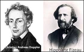
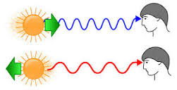
The Doppler effect is the frequency change of a periodic phenomenon induced by the movement of the emitter with respect to the receiver. In the case of sound waves, for example, the sound emitted by an approaching car is sharper than the sound emitted when it moves away.
Let us take the general case in Restricted Relativity of a light wave propagating at the wave speed c.
If f is the frequency of the wave perceived by an Observer O of a reference frame R, then any Observer O' of the reference frame R' in uniform rectilinear translation of velocity v with respect to R will perceive this same wave at a frequency f' different from f. The expression of f' is the following in different cases.
u is the unit vector of the light propagation MO (see Figure in Aberration).
γ is the Lorentz facteur
(D1) Longitudinal Doppler effect (u parallel to v) :
f' = f γ (1 - (v.u)/c)
When v is small compared to c, we find the approximate non-relativistic formulas :
f' = f (1 - (vr.u)/c) for mobile receiver (velocity vr) and immobile emitter with respect to the propagation medium
f' = f / (1 - (ve.u)/c) for immobile receiver and mobile emitter (velocity ve = -v) with respect to the propagation medium
f' = f (1 - (vr.u)/c) / (1 - (ve.u)/c) for mobile receiver (velocity vr) and mobile emitter (velocity ve) with respect to the propagation medium (relative velocity vr - ve = v).
(D2) Transverse Doppler effect at the emission (u perpendicular to v dans R) :
f' = f γ
(D3) Transverse Doppler effect at the reception (u perpendicular to v dans R') :
f' = f γ-1
(D4) Doppler effect (general formula) :
If the light propagation u makes with the velocity v an angle θ in R and θ' in R' (see Figure in Aberration), then we have the relation :
|
f' = f γ (1 - cos[θ] v/c) = f γ-1 (1 + cos[θ'] v/c)-1 |
the relation between the angles θ and θ' being given by the Aberration formula.
For θ = θ' = 0 or 180 , we find the formula (D1) with shift directed towards red or blue according to whether the Observer of R' moves away or approaches the light source of R.
For θ = 90 , we find the formula (D2) with shift directed towards blue.
For θ' = 90 , we find the formula (D3) with shift directed towards red.
When v is small compared to c, we find the approximate non-relativistic formula :
f' = f (1 - (vr.u)/c) / (1 - (ve.u)/c) for mobile receiver (velocity vr) and mobile emitter (velocity ve) with respect to the propagation medium (relative velocity vr - ve = v).
|
Partial proof [ANN Electricité_2] : Longitudinal Doppler effect (see Figure in Lorentz-Poincaré Transformation) : The equation of the light wave propagating in the direction Ox is as follows for the Observer bound to R : s(x, t)= s0 cos[ 2 π f (t - x/c) ] For the Observer bound to R', it becomes s(x', t') using the inverse Lorentz-Poincaré transformation : (L1') x = γ (x' + v t') (L2') t = γ (t' + B x') (L3) γ = 1 / (1 - v2 c-2)1/2 (L4) B = v c-2 So : s(x', t')= s0 cos[ 2 π f γ (t'(1 - v/c) + x'(B - 1/c)) ] The frequency f' perceived is thus : f' = f γ (1 - v/c) The longitudinal Doppler effect is called first order because it depends on (1 - v/c). It causes a decrease in frequency for v > 0 (leakage of the Observer with respect to the wave) and an increase in the opposite case. Transverse Doppler effect at the emission (see Figure in Lorentz-Poincaré Transformation) : The equation of the light wave propagating in the direction Oy is the following for the Observer bound to R : s(y, t)= s0 cos[ 2 π f (t - (y/c)) ] For the Observer bound to R', it becomes s (x', y', t') using the inverse Lorentz-Poincaré transformation : (L0') y = y' (L2') t = γ (t' + B x') So : s(x', y', t')= s0 cos[ 2 π f γ (t' + B x' - γ-1 (y'/c)) ] The frequency f' perceived is thus : f' = f γ The transverse Doppler effect is called second order. |
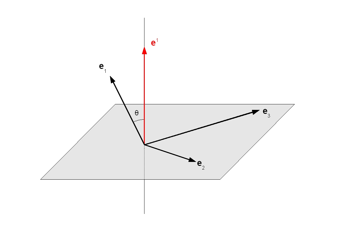
The dual space E* of a vector space E is the space of coordinated Linear forms on E.
E* is also a vector space and of same dimension (n) as E.
If ej are the basic vectors of E and ei the basic vectors of E*, then we have the following relations :
|
ei.ej = δij |
where δ is the Kronecker symbol
|
Proof : Let ei(x) be the linear application that matches the vector x to its component xi in base {ej}, what is written : ei(x) = xi For each index i ranging from 1 to n, ei(x) is therefore a Linear form on E, called the ith coordinated linear form relative to the base {ej}, what is written : ei(ej) = δij Fréchet-Riesz representation theorem : if ei is the vector representing the Linear form ei(x) for the Scalar product, then it can be written for any x of E : ei.x = ei(x) Hence the result : ei.ej = ei(ej) = δij |
Any vector x is therefore expressed in each base as follows :
x = xi ei
x = xi ei
where xi and xi are respectively the Covariant and contravariant components of the vector x.
|
Proof of covariant components : The first expression (x = xi ei) induces that : x.ej = (xi ei).ej = xi δij = xj which is indeed the definition of the covariant components xj of the vector x. |
Geometric interpretation (see Figure above) :
The vector ei is orthogonal (with respect to the Scalar product) to all vectors ej having different index j (ei.ej = 0) and has a scalar product equal to 1 with the vector ej having the same index (ei.ei = 1).
Properties :
ei = gij ej
ei = gij ej
where gij and gij are respectively the direct and inverse components of Metric tenseur
|
Proof : For any x, it can be written : ei.x = ei.(xj ej) = gij xj = gij ej(x) = gij ej.x Hence the first result : ei = gij ej By multiplying the two members of this relation by gki and using the relation gki gij = δkj, we find : gki ei = δkj ej = ek Hence the second result : ei = gij ej |
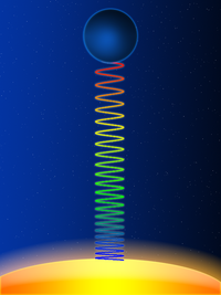
A frequency produced by a light source in a gravitational field is decreased (red shifted) when it is observed from a place where gravity is less. This is a pure General Relativity effect and not a shift by Doppler effect.
This phenomenon, predicted in 1915 by Albert Einstein, was observed in 1960 by Pound and Rebka.
By using the Schwarzschild metric centered on a massive mass (mass M) with spherical symmetry, and in the particular case of a zero Cosmological constant and a gravitational field in vacuum, the observed frequency f' at the radial distance r' is a function of the produced frequency f at the radial distance r according to the law :
|
f' = f ( (1 - r*/r)/(1 - r*/r') ) 1/2 |
where r* is the gravitational radius (r* = 2 G M c-2).
When the Observer is situated in a place of gravitation less than the source place (r' > r), we find (f' < f) corresponding to the observation of a shift directed towards red.
The Einstein effect has an impact in everyday life : if it were not taken into account in the gravitational Earth field, the GPS positioning system would be completely inoperative !
The Einstein tensor is the Tensor with the expression : Rab - (1/2) gab R
It corresponds to the first member of the Modified Einstein tensor without the term of the cosmological constant (Λ gab).
The notations are those in Maxwell Equations.
In Restricted Relativity, the Lorentz force (F_LORENTZ = q (E + v x B)) is written in a tensorial form whose components are the following [GOU, Relativité Restreinte, p.538] :
|
fi_LORENTZ = q Fij uj |
where f_LORENTZ is the Quadri-force of Lorentz and u is the Quadri-velocity of the particle.
Fij is the electromagnetic tensor. It is a Antisymmetric Tensor of order 2.
In Cartesian coordinates, all the components are of dimension m-1.V or C-1.N or kg.m.s-3.A-1.
In the Local reference frame of the Observer, and according to the Signature convention (-, +, +, +), these components are written [GOU, Relativité Restreinte, p.541] as follows :
|
Fij = -δ0i Ej + Ei δ0j + c ε0kij Bk or in matrix form : Fii for i ≥ 0 = 0 Fi0 for i > 0 = -F0i = Ei F21 = -F12 = -c B3 F31 = -F13 = c B2 F32 = -F23 = -c B1 |
where :
Ei = spatial components of the electric field E
Bi = spatial components of the magnetic field B
δij = Kronecker symbol
εijkl = Levi-Civita symbol with 4 indexes
By index increasing (see Elementary tensor operators), we find the components of the Tensors Fij and Fij in the following form :
Fij = gik_MINK Fjk
Fii for i ≥ 0 = 0
Fi0 for i > 0 = F0i = Ei
F21 = -F12 = -c B3
F31 = -F13 = c B2
F32 = -F23 = -c B1
Fij = gil_MINK Fjl
Fii for i ≥ 0 = 0
Fi0 for i > 0 = -F0i = -Ei
F21 = -F12 = -c B3
F31 = -F13 = c B2
F32 = -F23 = -c B1
gij_MINK are the inverse components of the Minkowski metric.
Let U, V and T be Tensors of arbitrary order and valence bearing on the indexes i, j, k, l...
Using the Convention of summation, the following elementary operations are defined on these Tensors :
|
- Sum (Tijk = Uijk + Vijk) of components : Tijk = Uijk + Vijk - Product by a scalar s (Tijk = s Uijk) of components : Tijk = s Uijk - Scalar product (T = Uij.Vkl) of component : T = Uij Vij - Tensor product (Tijkl = Uij ⊗ Vkl) of components : Tijkl = Uij Vkl - Partial derivative of the components Uij of a Tensor : d(Uij)/d(xk) = Uij,k - Covariant derivative (DkUij or Uij;k) - Divergence (Divi(Uij) or Uij;i) - Index increasing : Uik = gij Ujk - Index lowering : Uik = gij Uik - Index contraction : Uijk contracted on j and k = Uikk - Base change Warning : Classic partial derivative of a Tensor (example : Uij,k) is not generally a Tensor. Only the Covariant derivative is (example : Uij;k). |
Energy E and impulse vector P of a particle M, mesured by an observateur O in his Local reference frame at time τ, are given by the following relations (see Figure above) [GOU, Relativité Restreinte, p.275 to 278] :
|
E = -c p.u0 = γ m c2 A P = p - (E/c) u0 = γ m B A = 1 + a0.OM B = v + ω xu0 OM |
L, p and m are the Universe line, Quadri-impulse and mass at rest (or proper mass) of the particle.
L0, u0 and a0 are the Universe line, Quadri-velocity and quadri-accelaration of the Observer.
γ is the Lorentz facteur
ω is the Quadri-rotation of the Observer O.
v is the velocity of point M with respect to the Observer O in his Local rest space Eu0.
"xu0" is the Cross product operator between two any vectors of Eu0, what is written : ω xu0 OM = Ε(u0, ω, OM, .)
where :
Ε is the Levi-Civita tensor
Ε(u0, ω, OM, .) is the vector representing the Linear form Ε(u0, ω, OM, z) for the Scalar product g.
The impulse vector P (of dimension kg.m.s-1) is the orthogonal projection of vector p on Eu0 (with P.u0 = 0).
The energy E (of dimension J or kg.m2.s-2) satisfies the Einstein relation : E2 = m2 c4 + P.P c2 which is simplified in : E = ||P|| c for a particle of zero mass (case of photon for example).
|
Proof : p.p = (E/c)2 u0.u0 + 2 (E/c) P.u0 + P.P = -(E/c)2 + 0 + P.P We have moreover : p.p = -m2 c2 Hence the following result : E2 = m2 c4 + P.P c2 |
When L crosses L0 at the proper time τ0 (OM = 0) or when O is an inertial observer (a0 = ω = 0), these relations are simplified by :
|
E = γ m c2 P = γ m v γ = ( 1 - c-2 v.v )-1/2 |
The first relation expresses the equivalence between mass and energy. It was established in 1905 by Einstein [EIN Ist die Trägheit], a few months after his founding article on Restricted Relativity.
This relation can be written : E = Emass + Ecin, where Emass is the mass energy (Emass = m c2) and Ecin the kinetic energy of the particle (Ecin = (γ - 1) m c2).
In non-relativistic limit (||v|| << c) with limited development of γ, it is found that : Ecin = (1/2) m v.v and : P = m v
Mass-energy equivalence was indirectly confirmed in the 1930s-1940s by numerous experiments in nuclear and particle physics, then confirmed in 2008 by the international team of the "Centre de Physique Théorique de Marseille" by showing that the mass of the proton comes from the energy of quarks and gluons.
The Energy-impulse tensor (Tab) can take very varied forms depending on the distribution of matter or energy. For example : the tensor of the perfect fluid or that of electromagnetism.
Its components have the following meaning [GOU, Relativité Générale, p.112] :
|
T00 : energy density measured by the Observer T0j for j > 0 : (-c) times the component i of the relativistic impulse density (density of linear momentum) or (-1/c) times the component i of the energy flow (Poynting vector φ for electromagnetic field), measured by the Observer Tij for i and j > 0 : spatial components of the stress tensor (Sij) measured by the Observer |
It is a tensor of order 2, Symmetric and constructed so that its zero Divergence (Tab;a = 0) expresses in Continuum mechanics the two laws of conservation of impulse and energy (3 equations for the impulse vector and an equation for the energy).
In Cartesian coordinates, all the components are of dimension N.m-2 or kg.m-1.s-2
The notations are those in Maxwell Equations.
The components of the Energy-impulse tensor (Tij_EM) of ElectroMagnetic field are the following [GOU, Relativité Restreinte, p.635] :
|
Tij_EM = ε0 (Fim Fmj - (1/4) gij Fkl Fkl) |
where Fij is the Electromagnetic tensor.
In Restricted Relativity (Minkowski metric), the calculations give in Cartesian coordinates [GOU, Relativité Restreinte, p.636] :
T00_EM = energy density = (1/2) ε0 (E.E + c2 B.B)
Ti0_EM = T0i_EM for i > 0 corresponding to (-1/c) times φ with φ = Poynting vector = (1/ μ0) E x B
Tij_EM for i and j > 0 corresponding to Sij = ε0 ( (1/2) (E.E + c2 B.B) δij - (Ei Ej + c2 Bi Bj) )
where δ is the Kronecker symbol.
Properties :
The trace T_EM of the tensor Tij_EM is zero as follows : T_EM = gij Tij_EM = ε0 (Fim gij Fmj - (1/4) gij gij Fkl Fkl) = ε0 (Fim Fim - (1/4) 4 Fkl Fkl) = 0
A fluid is called "perfect" when the viscosity and thermal conduction effects can be neglected, which is the case in cosmology where the Universe expansion is assumed to be adiabatic (without heat exchange with the outside).
The components of the Energy-impulse tensor (Tij_FP) of Perfect Fluid are the following [GOU, Relativité Générale, p.114] :
|
Tij_PF = (ρ c2 + p) ui uj + p gij |
where :
ρ c2 and p represent respectively the energy density and the pressure of the fluid, both measured in the reference frame of the fluid.
u is the unit field which represents at each point the Quadri-velocity of a fluid particle (with ui = gik uk and uj = gjk uk).
When the Observer is Comoving with the fluid, the calculations give in Cartesian coordinates [GOU, Relativité Générale, p.114] :
T00_PF = ρ c2
Ti0_PF for i > 0 = T0i_PF = 0
Tij_PF for i and j > 0 corresponding to Sij = p δij
where δ is the Kronecker symbol.
The Perfect Fluid satisfies the low energy condition when : (ρ ≥ 0) and (ρ c2 + p ≥ 0), and the dominant energy condition when : (ρ c2 ≥ |p|).
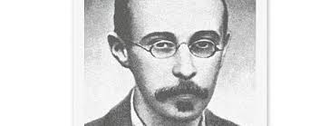
See Solution of Einstein Field Equation with Friedmann-Lemaitre-Robertson-Walker metric
Figures above from left to right : Alexander Alexandrowitsch Friedmann, Georges Lemaître, Howard Percy Robertson and Arthur Geoffrey Walker
The Friedmann-Lemaitre-Robertson-Walker metric is a Relativistic metric corresponding to a spatially homogeneous and isotropic Space-time.
In spherical coordinates (r > 0, colatitude θ = [0, π], longitude φ = [0, 2 π]) (see Figure in Space-time), the metric is written as follows for any coordinate system (ct, r, θ, φ) and by taking the Signature convention (-, +, +, +) :
|
ds2 = -c2dt2 + a(t)2 ( dr2 (1 - k r2)-1 + r2 (dθ2 + sin2[θ] dφ2) ) |
where k is a constant called space curvature parameter that can be flat (k = 0), closed (k = 1) or open (k = -1) ;
and a(t) is a function of t only, called scale factor or curvature factor or universe radius (a(t) > 0).
The coordinate r is dimensionless and the radius (a) has the dimension of a length.
The case k = 0 corresponds to a flatness of spatial sections and not of Space-time.
The gravitational potentials gij then are the following :
|
g00 = -1 ; g11 = a(t)2 (1 - k r2)-1 ; g22 = a(t)2 r2 ; g33 = a(t)2 r2 sin2[θ] ; gij = 0 for i and j taken different between 0 and 3 with a(t) = solution of a differential equation (see Solution of Einstein Field Equation with Friedmann-Lemaitre-Robertson-Walker metric). |
The sign of d(a)/dt informs about the universe evolution : positive if expansion, negative if contraction and zero if static.
The spatial coordinates (xi) then describe spatial hypersurfaces of Euclidean type (for k = 0), hyperspherical type (for k = 1) and hyperbolical type (for k = -1), whose the spatial curvature k* is constant and is equal to : k* = 6 k a(t)-2
|
Proof of metric ds2 [GOU, Relativité Générale, p.194] : A spatially homogeneous and isotropic Space-time is equivalent to a maximally symmetric space of dimension 3 (or spatially constant curvature k*) with three possible types of maximally symmetric spaces according to the value of k* (not proofed here): If k* = 0, space is the space R3 provided with the standard Euclidean metric. Its metric is the following : gij dxi dxj = dr2 + r2 (dθ2 + sin2[θ] dφ2) If k* > 0, space is the hypersphere S3 which is the part of R4 defined by : x2 + y2 + z2 + w2 = 1 where (x, y, z, w) denotes a generic element of R4. This definition is the three-dimensional transposition of the definition of the two-dimensional sphere S2 in R3. Its metric is the following : gij dxi dxj = dΧ2 + sin2[Χ] (dθ2 + sin2[θ] dφ2) with Χ = [0, π] If k* < 0, space is the hyperbolic space H3 which is the upper sheet of the two-sheeted hyperboloid of dimension 3 defined in R4 by : x2 + y2 + z2 - w2 = -1 Its metric is the following : gij dxi dxj = dρ2 + sinh2[ρ] (dθ2 + sin2[θ] dφ2) with ρ > 0 By setting r = sin[Χ] = sinh[ρ], these three metrics are written in a common form : gij dxi dxj = dr2 (1 - k r2)-1 + r2 (dθ2 + sin2[θ] dφ2) with k = 0 for Euclidean space, k = 1 for the hypersphere and k = -1 for hyperbolic space. |
See Lorentz-Poincaré transformation
For a given Relativistic metric a geodesic is the curve (or trajectory) of the shortest distance between two given points.
Geodesics thus describe the movement of free particles (material systems or photons), that is when they are not subjected to an external force other than gravitation in the context of General Relativity.
John Archibald Wheeler, American specialist of General Relativity, says : "Matter tells space-time to bend and space-time tells matter how to move".
If we choose to parameterize the trajectory by the proper Time τ of the particle satisfying to : ds2 = -c2 dτ2, the geodesic tensor equations are written as follows [GOU, Relativité Générale, p.48] :
|
(d2xi / dτ2) + Γilk (dxk/dτ) (dxl/dτ) = 0 where Γijk are the Christoffel symbols. |
If the Metric tensor g is known (and therefore Γ), this equation constitutes a system of 4 differential equations of the second order for the 4 functions xi. According to Cauchy theorem, this system admits a unique solution if the following initial conditions are fixed :
xi(0) = four arbitrary constants
(dxi/dτ)(0) = ui0
ui0 being four constants satisfying : gij ui0 uj0 = -c2
In Restricted Relativity (Minkowski metric) with Cartesian coordinates, the coefficients gij are all constant, which cancels all the Christoffel symbols. The equations of the geodesics are reduced to : d2xi / dτ2 = 0 whose solutions are the ordinary straight lines : xi(τ) = ai(τ) τ + bi
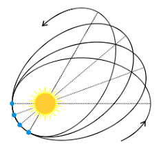
Trajectory :
The trajectory of a material body in a gravitational field with spherical symmetry (Schwarzschild metric) is a like-time Geodesic [GOU, Relativité Générale, p.71].
We suppose that the mass m of the material body is very small compared to the mass M of the central body of the Schwarzschild metric and that the Observer is placed in the equatorial plane z = 0 of the central body (θ = π/2, see Figure in Space-time).
The trajectory of the material body is flat and given by the following differential equation [GOU, Relativité Générale, pp80, 74, 72, 63, 64] :
|
dφ/dr = ±(1/r)2 (l/c) ( (ε/c2)2 - (1 + (1/r)2(l/c)2) (1 - r*/r) )-1/2 |
where :
r* = Schwarzschild radius (r* = 2 G M c-2)
M = mass of the central body
ε (in m2.s-2) = c2 (1 - r*/r) dt/dτ = -c2 ut.u = -c2 g00 u0
l (in m2.s-1) = r2 sin2[θ] dφ/dτ = c uφ.u = c g33 u3
lcrit = 31/2 r* c
u = Quadri-velocity of the material body
ut and uφ = vectors of the Natural base associated respectively with stationarity and azimuthal symmetry of the metric.
τ = proper Time of the material body.
Note that the two quantities ε and l are constant along the Geodesic.
In Newtonian limit (when the material body is infinitely far from the central body), ε and l can be interpreted as follows :
ε = c2 + E0/m = energy per unit mass of the material body, measured by a static Observer.
l = angular momentum (relative to the z axis) per unit mass of the material body, measured by a static Observer.
E0 = mechanical energy of the material body (sum of kinetic energy and gravitational potential energy).
According to the coupled values of l and ε, the trajectory of the material body is then as follows [DEV, Un peu de physique, Trajectoire d'une particule] :
In the case where : |l| < lcrit, the material body is irreparably attracted by the central body.
In the case where : |l| > lcrit, the material body avoids the central body by continuing its course or, on the contrary, goes into orbit around.
In the case of an orbit, the trajectory can be a perfect circle or a quasi-ellipse with advance of the periastron (see Figure above). At the Newtonian limit, the trajectory is a stable ellipse that verifies Kepler's laws.
|
Proof of stable ellipse : The Newtonian limit is to do : E0/m << c2 and r*/r << 1. By putting u = 1/r, the trajectory equation becomes : dφ/dr = ± l ( (2 E0/m + r* c2 u - l2u2 )-1/2 which integrates into : u = (1 + e cos[φ])/p with : p = l2/(G M) e = (1 + 2 (E0/m) l2/(G M)2)1/2 We can recognize the polar equation of the keplerian ellipse of parameter p and eccentricity e |
Periastron :
The periastron is the point of the trajectory closest to the central body (see Figure above).
The advance δφper of the periastron (at first order of r*/r) is as follows [GOU, Relativité Générale, p.82] :
|
δφper = 3 π r* / ( a (1 - e2) ) |
where :
a = half-major axis of the ellipse
e = eccentricity of the ellipse
In the case of the periastron advance around the Sun (perihelion) of the planet Mercury (with M_Sun = 1.9891 1030 kg, a_Mercury = 5.79 1010 m, e_Mercure = 0.206), we find : δφper = 5.0 10-7 rad. Since the orbital period of Mercury is 88 days, the cumulative effect after a century is : Δφper = 43"
This advance was observed as early as 1859 by Urbain le Verrier and and explained in 1915 by Albert Einstein [EIN Die_Grundlage].
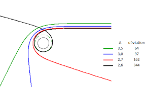
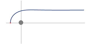
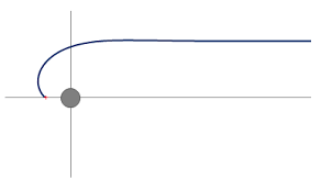
Figures above from left to right : Figure 1 = Deflection of light rays for large b ; Figures 2 to 4 from [DEV A little physics - Trajectory of a ray of light] = Deflection of light rays according to the value of b
Trajectory :
The trajectory of a photon in a gravitational field with spherical symmetry (Schwarzschild metric) is a like-light Geodesic [GOU, Relativité Générale, p.82].
We suppose that the Observer is placed in the equatorial plane z = 0 of the central body of the metric (colatitude θ = π/2, see Figure in Space-time).
The photon trajectory is flat and given by the following differential equation [GOU, Relativité Générale, p.85, 86] :
|
dφ/dr = ±(1/r)2 ( (1/b)2 - (1/r)2 (1 - r*/r) )-1/2 |
where :
r* = Schwarzschild radius (r* = 2 G M c-2)
M = mass of the central body
b = impact parameter for photons coming from infinity (see Figure 1 above)
bcrit = (3/2) 31/2 r*
In the case where : b > bcrit, the photons coming from infinity will approach the central body and return to infinity. The trajectory looks like a hyperbola for the large values of b (see Figure 1 above) and can make several rounds of the central body before starting again for the values of b near bcrit (see Figure 2 above).
In the case where : b ≤ bcrit, the photons are trapped by the central body and a distant Observer can not receive them (see Figures 3 and 4 above).
This differential equation is integrated in the following form which is solved as an elliptic integral [DEV Un peu de physique - Trajectoire d'un rayon lumineux].
|
φ = (r*)-1/2 Integral_from_0_to_u[du / F(u)1/2] u = 1/r F(u) = u3 - (r*)-1 u2 + (r*)-1 b-2 |
Periastron :
The periastron is the point of the trajectory closest to the central body (see Figure 1 above).
Its radius rper is given by the following equation [GOU, Relativité Générale, p.86] :
|
P(rper) = rper3 + 3 p rper + 2 q = 0 p = -(1/3) b2 q = (1/2) r* b2 |
This cubic equation is solved as follows :
|
- For b ≥ bcrit : rper = (2 / 31/2) b cos[(π - α)/3] with : α = cos-1[bcrit / b] Note that for b >> bcrit, we have : α = π/2 and we find : rper = b corresponding to no deflection of the photon away from the central body. - For b < bcrit : there is no periastron satisfying the relation : dr/dφ = 0 |
|
Proof : Let Q = p3 + q2 = (1 / 27) b4 (bcrit2 - b2) The study of the function P(rper) shows that : - For b > bcrit : there are three real roots, one of which is negative. The largest positive root corresponds to the periastron rper which is reached continuously from a photon arriving from infinity. Given the particular conditions : p < 0 and Q < 0, the cubic equation is resolved classically in trigonometric form [CHO Mathématiques] and gives for greater root : rper = 2 (-p)1/2 cos[(π - α)/3] with α = cos-1[q / (-p)3/2]. See Figure 2 above. - For b = bcrit : there is a positive double root (-q/p) corresponding to the periastron rper and a single negative root (2 q/p). The trajectory tangents the circle of radius equal to : bcrit / 31/2. See Figure 3 above. - For b < bcrit : there is only one real root, which is negative. So there is no periastron rper satisfying the relation : dr/dφ = 0. The trajectory converges towards the central body. See Figure 4 above. |
Deflection :
In the case where : b >> bcrit and at first order of r*/b, the deflection δφ of the light ray from a straight line path (see Figure 1 above) is then as follows [GOU, Relativité Générale, p.86, 87] :
|
δφ = 2 (r*/b) |
In the case of a trajectory skimming the Sun surface (b = R_Sun = 6.96342 108 m, with M_Sun = 1.9891 1030 kg), we find : r* = 3,0 103 m and δφ = 1.75"
This deflection, predicted in 1915 by Albert Einstein, was highlighted by Arthur Eddington and his team, measuring the stars position near the solar disk during the eclipse of 1919. It is this event that made Einstein famous among the general public.
The deflection of light rays is at the origin of the phenomenon of Gravitational mirage.
Apparent radius :
For an Observer located at infinity, the apparent radius Ra of a star of radius R and that of a Black hole of radius r* (considered to delimit its surface) then is [GOU, Relativité Générale, p.299, 300] :
|
For a star : Ra = R (1 - (r*/R))-1/2 For a Black hole : Ra = bcrit = (3/2) 31/2 r* |
The star always appears bigger than it is (Ra > R).
For the Black hole, the photons with low impact parameter (b < bcrit) are trapped by the Black hole and the Observer receives no photon. So he observes on the sky background a black disk of apparent radius almost three bigger than it is (Ra = 2.60 r*).
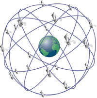
GPS (Global Positioning System), originally known as NAVSTAR System (NAVigation System by Timing And Ranging), is a very precise three-dimensional positioning system (latitude, longitude, altitude) with worldwide coverage, put into service in the 1970s-1980s by the United States Department of Defense (DoD).
GPS is relative to the worldwide WGS84 geodetic system (see Meteo - Appendix 2).
In 2024, in standard service (free), GPS provides an accuracy of 3 to 5 m horizontally and 5 to 8 m vertically.
The European GPS counterpart is the GALILEO system, operational since 2016.
GALILEO is relative to the European GTRF geodetic system which is compatible with WGS84 to less than 1 m.
In 2024, in standard service (free), GALILEO provides an accuracy of 1 m horizontally and 2 m vertically. The high-precision service (HAS), also free, accessible only to high-end receivers, provides an accuracy of 20 cm horizontally and 40 cm vertically.
Detail about GPS (cf [GOU, Relativité Générale, p. 203-205]) :
The GPS is based on a set of at least 24 satellites distributed 4 by 4 in 6 circular orbits of orbital period T = 12 h and radius rsat = 26561 km = 4.16 REarth (with REarth = 6378 km and MEarth = 5.97 1024 kg). See Figure above.
Each satellite (i) carries a cesium atomic clock and emits a radio signal including its emission date (ti) and its three spatial coordinates ri (deduced ephemeris related to its orbit).
Any Observer on Earth who receives at the same time (t) the signals of at least four satellites can then calculate his position r. If Space-time was flat (Minkowski metric), the observer should simply solve the system of 4 equations : ||r - ri|| = c (t - ti). But in reality, it is essential to consider three types of temporal shifts :
1. Imprecision of cesium atomic clocks :
To have a precision of one meter on the position r, it is necessary a precision on the dates ti of the order of 3 ns (dt = 1 m / c). The stability of cesium atomic clocks is such that : dt/t = 10-13. dt = 3 ns is thus reached in t = 10 h approximately. To achieve the required accuracy, the clocks are then adjusted several times a day using signals sent from the ground.
2. Durations dilation :
This durations dilation constitutes the transverse (second order) Doppler effect. The first-order Doppler effect in v/c affects only the signal frequency and not the content of the delivered message (date and position of the emitter).
As the satellites are moving relative to the observer, their orbital speed is : v = (G MEarth / rsat)1/2 = 3.87 km.s-1. Hence the result : dt/t = γ - 1 = 8.3 10-11 (where γ is the Lorentz factor). If no correction is applied, dt = 3 ns is reached in 30 seconds !
3. Einstein effect :
Since the satellites are four times higher than the observer on the ground, Einstein effect therefore applies with an offset : dt/t = G MEarth c-2 (1/REarth - 1/rsat) = 5.3 10-10
If no correction is applied, dt = 3 ns is reached in 6 seconds, which would correspond to a positioning error of 14 km in a day !
To take into account these two relativistic shifts, the proper frequency of the atomic clocks is corrected before the radio signal emission towards the Earth (see [GOU, Relativité Générale, p. 205, 211]).
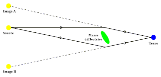
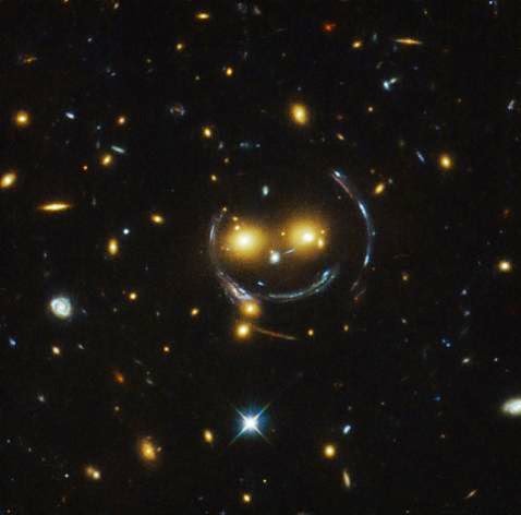
The deflection of light rays is at the origin of the phenomenon of gravitational mirage gravitational mirage, predicted in 1936 by Albert Einstein and observed in 1979 by Dennis Walsh and his colleagues Robert Carswell and Ray Weymann on the double quasar QSO 0957+561.
This phenomenon can take different aspects depending on the alignment of the Observer, the mass that deforms (galaxy for example) and the observed source (quasar for example). We can see perfect rings (called Einstein rings), circles arcs or simply images multiplied from the source (see Figures above).
Not only do these gravitational lenses deflect but amplify the deflected light, which fascinates astronomers.
When a massive object moves through space-time, the curvature of space-time adjusts to reflect the change in the object's position.
Under certain circumstances, accelerated objects can produce a disturbance in space-time that expands and propagates in a manner analogous to waves on the surface of water.
This type of disturbance is called a gravitational wave and is predicted to propagate at the light speed.
Albert Einstein predicted the existence of gravitational waves in 1916. Gravitational waves from the merger of two black holes were detected directly in 2015 by the LIGO laser (international collaboration).
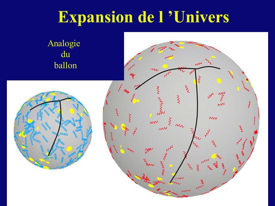
The expansion of the universe was predicted in 1922 by Alexander Friedmann.
The Hubble-Lemaître law stated in 1929 states that galaxies move away from each other at an expansion speed v approximately proportional to their distance d :
|
v = H(t) d |
where H(t) is the Hubble parameter used in particular in the Friedmann equations.
The value to date of H(t) (called Hubble constant H0) is about 70 (km/s)/Mpc, with 1 pc = 1 parsec = 3.2616 light-years = 3.085677581 1016 m
The speed v is not a physical speed. It only reflects the Space-time expansion which causes an global movement of the universe galaxies. The Earth thus "retreats before the light" because the Space-time expands.
Any distant galaxy having the same proper Time as the Observer (called Cosmic time), there is no relative time effect (Doppler-Fizeau effect) on its radiation period but a simple differential delay effect on the radiation period received.
The own movements acquired by the galaxies superimpose to this global movement because of their gravitational interactions with their neighbors.

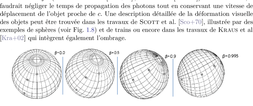
[GOU, Relativité Restreinte, p. 163-171]
- For the same Observer O at a fixed instant τ of his proper Time, we must not confuse the position (x, y, z) of an object M and its perceived image. This image or photograph is generated by all the photons arriving from M to O. The Lengths contraction concerns in particular the position of the object and not its image.
- For a cube that moves perpendicularly to the sight line of an Inertial observer, he perceives the image of a cube that has been rotated by a given angle θ (see Figure 1 above). He perceives the back face of the cube in addition to the face facing him. This apparent rotation is not relativistic and results from the finite time of light propagation. Relativity intervenes only through the contraction of the face oriented towards the observer according to the Lorentz-Poincaré Transformation.
- The image of a moving sphere is a sphere that seems to have undergone a rotation and presents its opposite face to the movement (see Figure 2 above). If we take into account only the finite time of light propagation in a (Galilean) non-relativistic theory, a sphere would appear elongated in the direction of the movement. It is thanks to the Lengths contraction that it appears exactly spherical. Only the angular size of the circle can change.
- Some astrophysical movements may be superluminous, with apparent speeds greater than c. These superluminous apparent speeds are generated by subluminic movements in a direction close to the sight line. Thus the micro-quasar GRS 1915+105 was observed in 1994 in our galaxy with an apparent speed 1.25 c corresponding to an material ejection at the speed 0.92 c at an angle θ of 70 .
The contraction operation of the index of a mixed component of a Tensor consists in choosing two indexes, one covariant and the other contravariant, then in equalizing and summing them with respect to this twice repeated index.
For example, for a Tensor U of order 3 whose mixed components are Uijk, the contraction on the indexes j and k gives the Tensor Ti = Uikk = Ui11 + Ui22 + ... Uinn
The quantities Ti (contracted components of the tensor U) form the components of a tensor T of order 1.
Note that the "matrix product" operator is a particular case of the Tensor product Uij ⊗ Vkl contracted in the form : Til = Uik Vkl
Another examples :
Case of the Curvature tensor Rijkl : the contraction on the indexes i and k gives the Ricci tensor : Rjl = Rkjkl
Warning : If the same letter is kept for the resulting tensor (after deletion of the identical indexes), then the notation may become ambiguous. For the Tensor Rijlk (different from Rijkl), the contraction on the indexes i and k gives the Tensor Rkjlk = Rjl, i.e. the opposite of the Ricci Tensor despite the identical notation Rjl.
Case of the Curvature tensor Rijkl : the Index increasing of the index i gives, after contraction on the indexes m and i, the Tensor gmi Rijkl = Rmiijkl = Rmjkl
Warning : If the same letter is kept for the resulting tensor (after deletion of the identical indexes), then the notation may become ambiguous. For the Tensor Rjikl (different from Rijkl), its contraction with gmi gives the Tensor gmi Rjikl = Rmijikl = Rmjkl, i.e. the opposite of the Tensor Rmiijkl despite the identical notation Rmjkl.
A lower index can be changed to a higher index by multiplication with the inverse Metric tensor gij then Index contraction. Examples :
Uik = gij Ujk
Uik = gil gkm Ulm
Warning : If the same letter is kept for the resulting tensor (after deletion of the identical indexes), then the notation may become ambiguous (see Index contraction).
A higher index can be changed to a lower index by multiplication with the Metric tensor gij then Index contraction. Examples :
Uik = gij Ujk
Ulm = gjl gkm Ujk
Uklm = glp Ukpm
Warning : If the same letter is kept for the resulting tensor (after deletion of the identical indexes), then the notation may become ambiguous (see Index contraction).
In classic physics, an inertial reference frame (called "stationary system" by Einstein [EIN Zur_Elektrodynamik]) is a reference system in which the inertia principle is verified, that is to say that any free material body (on which the resultant forces is zero) is in rectilinear translational movement (without rotation) with uniform speed, the immobility being a special case.
A material body in rotational movement or non-rectilinear translational movement or non-uniform speed constitutes a non-inertial reference frame.
In Restricted Relativity, a body (or Observer) is called "inertial" when its Local reference frame is constant along its Universe line, i.e. it verifies the following relation [GOU, Relativité Restreinte, p.91, 92] :
|
d(eα)/dτ = 0 |
where τ is the proper Time of the body
eα are the four basic vectors of the Local reference frame linked to the body.
A body is called "inertial" also when both its trajectory is a straight line of Minkowski's Space-time (zero quadri-acceleration a) and its Quadri-rotation ω is zero.
a and ω are quantities measurable by the observer contrary to his Quadri-velocity u [GOU, Relativité restreinte, p.90].
The expression of the Kronecker symbol δ is as follows :
|
δij = δij = δij = 1 for i = j and 0 otherwise. |
Warning : the Kronecker symbol is not a Tensor. For example, the index lowering : δij = gik δkj is not possible, which is false considering that : gik δkj = gij
Property :
Index replacement in any Tensor T : Tjk = δij Tik
In Restricted Relativity, if a bipoint of given proper length (l0) is fixed in a reference frame, then its length in any other reference frame is less than the proper length and is called apparent length (l).
Some authors talk about Lengths contraction. This contraction is not physical but simply results from measurements that only make sense with respect to a given reference frame.
The lengths contraction intervenes only in the direction of the relative movement between reference frames. There is no contraction in the orthogonal directions.
This phenomenon was demonstrated indirectly by Bruno Rossi and David B. Hall via the cosmic muon experiment.
|
Proof of relation : l < l0 in Restricted Relativity [ANN Electricité_2] : Let a fixed rigid bar in the reference frame R. Its extremities are respectively at coordinates (x1, y1, z1) and (x2, y2, z2). Its (own) length l0 is such that : l02 = (x2 - x1)2 + (y2 - y1)2 + (z2 - z1)2 For an Observer of the reference frame R' in uniform rectilinear translation at the speed v with respect to R, which locates the bar extremities at the same time t', he finds coordinates (x1', y1', z1') and (x2', y2', z2') given by the inverse transformation of Lorentz- Poincaré : x1 = γ (x1' + v t') y1 = y1' z1 = z1' x2 = γ (x2' + v t') y2 = y2' z2 = z2' The (apparent) length l of the bar for this observer is therefore such that : l2 = (x2' - x1')2 + (y2' - y1')2 + (z2' - z1')2 = (x2 - x1)2 γ-2 + (y2 - y1)2 + (z2 - z1)2 = l02 - (x2 - x1)2 (1 - γ-2) = l02 - (x2 - x1)2 (v/c)2 So : l < l0 |
The expression of the Levi-Civita symbol ε is as follows (not to be confused with the Levi-Civita tensor) :
|
εijkl... = εijkl... = 0 if two or more indexes (i,j,k,l...) are equal +1 if (i,j,k,l...) is an even permutation of (0,1,2,3...) -1 if (i,j,k,l...) is an odd permutation of (0,1,2,3...) |
When any two indexes are interchanged, equal or not, the symbol is negated : ε...i...l... = -ε...l...i...
For 3 indexes (i,j,k) we have :
εijk = +1 for 012 or 120 or 201
εijk = -1 for 021 or 102 or 210
For 4 indexes (i,j,k,l) we have :
εijkl = +1 for 0123 or 0231 or 0312 or 1032... or 3210
εijkl = -1 for 0132 or 0213 or 0321 or 1023... or 3201
ε allows to express many vectorial operations in a compact form. In a vector space of dimension 3 and with the Convention of summation, it can be written for example :
- Cross product (w = u x v) of components : wi = εijk uj vk
- Curl (w = curl(u)) of components : wi = εijk uk,j
- Determinant (d = det(u,v,w)) of component : d = εijk ui vj wk = εijk ui vj wk
The Levi-Civita tensor Ε is a Tensor of order 4 which is written as follows, for any quadruplet of vectors (u, v, w, z) [GOU, Relativité Restreinte, p.20, 21, 482 to 487] :
|
Ε(u, v, w, z) = μ (-g)1/2 εijkl ui vj wk zl μ = 1 or -1 depending on whether the base is respectively Direct or indirect g = Determinant of the matrix gij associated with Metric Tensor g εijkl = Levi-Civita symbol with 4 indexes |
Its 256 components in any base {ei} are as follows :
|
In covariant components : Εijkl = μ (-g)1/2 εijkl In contravariant components : Εijkl = -μ (-g)-1/2 εijkl |
Properties :
- Ε is Antisymmetric (or alternating) : the quantity Ε(u, v, w, z) is 0 when two of its arguments are equal. For example : Ε(u, v, u, w) = 0
- In any Orthonormal and Direct base : Ε(u, v, w, z) = det(u, v, w, z)
- Ε only has one independent component Ε0123 = μ (-g)1/2
- The quantity (Εijkl Εijkl) is egal to -24
- If ei are the basis vectors : Ε(e0, e1, e2, e3) = μ (-g)1/2
- In any Orthonormal base : Ε(e0, e1, e2, e3) = μ
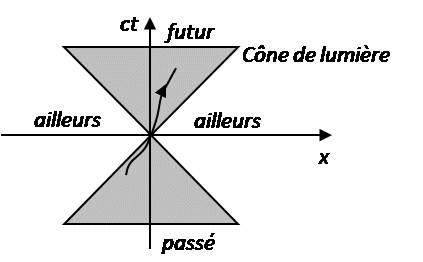
The light-cone is a fundamental notion of Restricted Relativity allowing the distinction between a past event, a future event and an inaccessible event (in the past or in the future).
If a light signal starts from origin point O to point M of coordinates (x, y, z), then the set of trajectories of the light rays from O in the Space-time will be a hypercone of equation : c2 t2 = x2 + y2 + z2, called Light-cone (see Figure above where x represents in a simplified way the three spatial coordinates x, y and z).
Figures above from left to right : René Maurice Fréchet and Frigyes Riesz
Any linear form ω is an application that matches a number ω(u) to any vector u, and this in a linear way [GOU, Relativité Restreinte, p.21] :
|
For any scalar λ and any vectors u and v : ω(λ u + v) = λ ω(u) + ω(v) |
ω(u) is sometimes noted <ω, u> with the bra-ket notation as in quantum mechanics.
Examples : if a and b are vectors of a vector space E, the linear applications that match the vector u respectively to the scalars u.a and det(u, a, b) are both linear forms.
Properties :
- There is only one vector w that represents the Linear form ω of the Dual space (E*) for the Scalar product.
- The vector w satisfies the relation : w.z = ω(z) for any vector z
- In any base {ei} of E, its Covariant components are written : wi = w.ei = ω(ei) and its contravariant components are written : wi = gij wj = gij ω(ej) = ω(gij ej) = ω(ei)
- Notation [GOU, Relativité Restreinte, p.87, 538] : The vector w is sometimes noted : w = ω(.)
|
Proof : Let E be a vector space with its Scalar product and ω a linear form continuous on E. So there is only one vector w of E such that we have the relation : w.z = ω(z) for any vector z of E (Fréchet-Riesz representation theorem). |
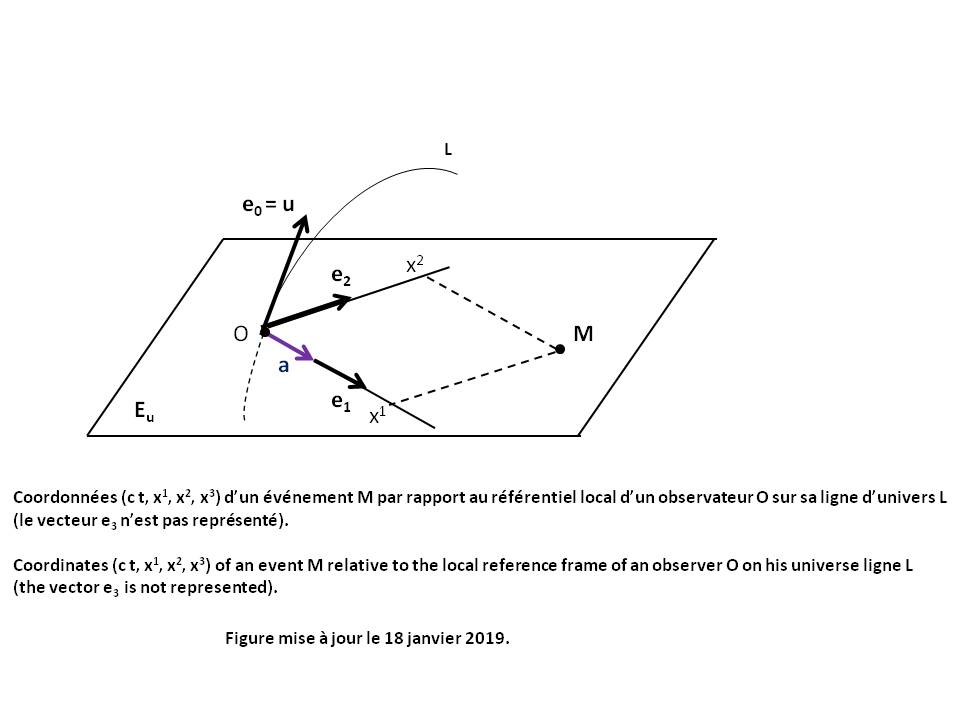
In Restricted Relativity, the local reference linked to a body (or Observer O) along its Universe line is a quadruplet of vectors (e0, e1, e2, e3) defined in any point (or event) of this Universe line and satisfying the following properties [GOU, Relativité Restreinte, p.60, 79, 80] :
- (e0, e1, e2, e3) is an Orthonormal and Direct base, called Serret-Frenet tetrad.
- e0 is tangent to the Universe line of the body (condition : e0 = u), where u is the Quadri-velocity of the body.
- the field (e0, e1, e2, e3) is class C1, i.e. the base (e0, e1, e2, e3) varies infinitesimally when we passe from a given point to a neighboring point on the Universe line.
The three vectors e1, e2 and e3 are therefore orthogonal to e0 = u. They belong to the Local rest space Eu of the Observer O (see Figure above).
Note that e1 can be choosen tangent to the curvature a of the Universe line of the body (condition : e1 = a/||a||), where a is the quadri-acceleration of the body. The length 1/||a|| is called curvature radius of the Universe line at point O.
Properties :
d(e0)/dτ = c a
d(e1)/dτ = c ||a|| e0 + c T1 e2
d(e2)/dτ = -c T1 e1 + c T2 e3
d(e3)/dτ = -c T2 e2
τ is the proper Time of the body
T1 and T2 are respectively the first and the second torsion of the Universe line of the body.
Let an Observer O of Universe Line L and Quadri-velocity u (see Figure above).
His local rest space is the vector hyperplane Eu orthogonal to u.
Let an Observer O of Universe Line L0 and Quadri-velocity u0 (see Figure above).
Let a particle M of Universe Line L and Quadri-velocity u.
It is assumed that L is situated in the neighborhood of L0, in the sense that L can be described in the Local reference frame of O, which means that the spatial distance between L0 and L is always much smaller than ||a0||-1, where a0 is the Quadri-acceleration of O.
Let an infinitesimal increment dτ0 of the Proper time τ0 of O and dτ the Proper time of the particle when it moves from M(τ0) to M(τ0 + dτ0) along its universe line.
The Lorentz factor γ of the particle M with respect to the Observer O is defined by the following relation [GOU, Relativité Restreinte, p.99 à 109] :
|
dτ0 = γ dτ |
The following relations are then demonstrated :
|
γ = -u0.u / A = ( A2 - c-2 B.B )-1/2 u = γ ( A u0 + c-1 B ) A = 1 + a0.OM B = v + ω xu0 OM |
ω is the Quadri-rotation of the Observer O.
v is the velocity of point M with respect to the Observer O in his Local rest space Eu0.
"xu0" is the Cross product operator between two any vectors of Eu0, what is written : ω xu0 OM = Ε(u0, ω, OM, .)
where :
Ε is the Levi-Civita tensor
Ε(u0, ω, OM, .) is the vector representing the Linear form Ε(u0, ω, OM, z) for the Scalar product g.
When L crosses L0 at the proper time τ0 (OM = 0) or when O is an inertial observer (a0 = ω = 0), these relations are simplified by :
|
γ = -u0.u = ( 1 - c-2 v.v )-1/2 u = γ ( u0 + c-1 v ) |
When L crosses L0 at the proper time τ0 (OM = 0) or when the Quadri-acceleration a0 of O is zero (in particular if O is an Inertial observer (a0 = ω = 0), then it is proved that : γ ≥ 1. Given the definition of γ as ratio of two proper durations, this property is called Durations dilation.
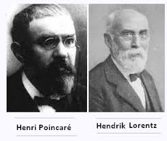
See Lorentz-Poincaré transformation
The main mathematical notations used in this page are as follows :
Elementary tensor operators :
Operators synthesis
, d grad div rot Δ Δ ◊ : Convention of partial derivative
akm bm ck : Convention of summation (called "Einstein convention")
; : Covariant Derivative
Div : Divergence
* : Dual (space and base)
. ||x|| : Scalar product and norme
⊗ : Tensor product
x : Cross product
Greace alphabetic symbols :
Λ : Cosmological constant
γ : Lorentz factor
ω : Linear form
η : Minkowski matrix
Γ : Christoffel symbols
δ : Kronecker symbol
ε : Levi-Civita symbol
ε0 : Dielectric permittivity in the vacuum
Latin alphabetic symbols :
a : Universe Radius
c : Light speed in the vacuum
Ε : Levi-Civita tensor
Eu : Local rest space of the observer
F : Electromagnetic tensor
g : Metric tensor
G : Universal gravitational constant
K : Gravitational coupling coefficient
k : Spacially constant curvature
O : Observer
R : Ricci tensor
R : Scalar curvature
r* : Gravitational radius
S : Modified Einstein tensor
T : Energy-impulse tensor
Non-relativistic electromagnetism :
Any particle of charge q and velocity v, subjected to an electric field E and to a magnetic field B, undergoes the Lorentz force F_LORENTZ = q (E + v x B)
The equations of James Clerk Maxwell specify the evolution of electromagnetic fields E and B. In vacuum with sources (point electric charges and/or their electric powers), these fields writte as follows :
|
(R1) div(E) = ρ/ε0 (R2) curl(E) = -dB/dt (R3) div(B) = 0 (R4) curl(B / μ0) = J + ε0 dE/dt |
The two densities ρ and J are connected by the relation of the charges conservation (see proof below) :
(R5) div(J) + dρ/dt = 0
E is the electric field (in m-1.V or C-1.N or kg.m.s-3.A-1)
B is the magnetic field (in T or kg.s-2.A-1)
J is the Electric power density (in m-2.A)
v is the particle velocity (in m.s-1)
q is the electric charge (in C or s.A)
ρ is the Electric charge density (in m-3.s.A)
μ0 is the permeability of vacuum : μ0 = 4 π 10-7 kg.m.A-2.s-2
ε0 is the dielectric permittivity in vacuum such that :
(R0) ε0 = 1 / (μ0 c2)
c is the light speed in vacuum (c = 2.99792458 108 m.s-1
The operators used are the following :
v1.v2 and v1 x v2 : Scalar product and Cross product of any two vectors v1 and v2.
div(v) and curl(v) : divergence and curl of any vector v (see Convention of partial derivative).
Δ : Laplacian operator (see Convention of partial derivative).
◊ : Alembertian operator (see Convention of partial derivative).
Relativistic electromagnetism :
|
In Restricted Relativity (Minkowski Metric), it is proved that (cf [HER, Etude, pp. 24, 25][GOU, Relativité Restreinte, pp 585, 507]) : The two relations (R2) and (R3) are equivalent to the following tensor relation : (RR1) Fkl,m + Flm,k + Fmk,l = 0 The two relations (R1) and (R4) are equivalent to the following tensor relation : (RR2) Fkl,l = jk/ε0 where : Fij = Electromagnetic tensor j = quadri- electric power In General Relativity, it suffices to replace the Partial derivatives by Covariant derivatives to extend the validity of these relations to General Relativity, which gives (cf [BARRAU, Relativité générale, p.64][HER, Etude, pp. 24, 25][GOU, Relativité Restreinte, pp 585, 507]) : (RG1) Fkl;m + Flm;k + Fmk;l = 0 (RG2) Fkl;l = (-g)-1/2 ((-g)1/2 Fkl),l = jk/ε0 where : g = Determinant of the matrix gij associated with Metric Tensor g |
Electrical and magnetic potentials :
The Electric potential V and the Magnetic potential A are defined from relations (R2) and (R3) by the following relations (see proof below) :
(R6) rot(A) = B
(R7) -grad(V) = E + d/dt(A)
If A satisfies the relation (R6), then any potential A' = A + grad(Ψ) also satisfies (R6). The magnetic potential A is therefore determined at within the gradient of a scalar field Ψ.
Likewise if two electric potentials V and V' satisfie the relation (R7), then we can write :
-grad(V' - V) = d/dt(A' - A)
We can deduce :
grad(V' - V + d/dt(Ψ)) = 0
V' = V - d/dt(Ψ) + f(t)
The electric potential V is therefore determined at within a time function f(t).
Lorenz gauge condition :
Replacing of the relations (R6) and (R7) in relations (R1) and (R4) gives :
(Δ - c-2 d2/dt2)(V) = -ρ/ε0 - d/dt(C)
(Δ - c-2 d2/dt2)(A) = -μ0 J + grad(C)
C = div(A) + c-2 d/dt(V)
Since the potential A is determined at within the gradient of a scalar field ψ, we can arbitrarily write :
(R8) C = 0
This relation is called Lorenz gauge condition (of the Danish physicist Ludvig Valentin Lorenz, not to be confused with the Dutch physicist Hendrik A. Lorentz), which ultimately gives :
(R9) ◊(V) = -ρ/ε0
(R10) ◊(A) = -μ0 J
The three relations (R8), (R9) and (R10) constitute a group of equations that contain the same information as the Maxwell equations.
These relations are invariant by Lorentz-Poincaré transformation (see proof below). it is the same for the Maxwell equations.
Resolution of the equations :
In vacuum and without any source (ρ = 0 and J = 0), the relations (R9) and (R10) show that the electromagnetic field is described by two Alembert's equations called wave equations.
In the general case of a distribution of sources P located in a domain D carrying electric charges and currents, or whose density decreases sufficiently rapidly with distance, the solutions of the equations (R9) and (R10) are the following, with the additional conditions V(∞) = 0 and A(∞) = 0 :
(R11) V(M, t) = ∑D[ (1/ε0) (4 π/||PM||) ρ(P, t - ||PM||/c) dτ ]
(R12) A(M, t) = ∑D[ μ0 (4 π/||PM||) J(P, t - ||PM||/c) dτ ]
These solutions are called delayed potentials because the potentials values at a point M at a time t depend on those of the sources at all the points P at the previous instant (t - ||PM||/c).
Proofs :
|
Proof of the relation of the charges conservation : The divergence of the relation (R4) gives : 0 = div(J) + ε0 div(dE/dt) = div(J) + ε0 d/dt(div(E)) Replacing of the relation (R1) in this relation gives : (R5) div(J) + dρ/dt = 0 |
|
Proof of the electrical and magnetic potentials : The relation (R3) allows to write : (R6) rot(A) = B where A is a magnetic potential (non-unique vector). Replacing of this relation in (R2) gives : rot(E + d/dt(A)) = 0 There is therefore an electric potential V (non-unique scalar) such that : (R7) -grad(V) = E + d/dt(A) |
|
Proof of Maxwell equations invariance by Lorentz-Poincaré Transformation : Let the simplified case where the x' axis of the reference frame R' is parallel to the x axis of the reference frame R (see Lorentz-Poincaré Transformation). The relations (L1) and (L2) give by partial derivation : d/dx = (d/dx')(dx'/dx) + (d/dt')(dt'/dx) = γ ((d/dx') - (d/dt') β c-1) d/dy = (d/dy') d/dz = (d/dz') d/dt = (d/dx')(dx'/dt) + (d/dt')(dt'/dt) = γ ((d/dt') - (d/dx') β c) Since the potentials A and V derive from the quadri- electromagnetic potential A*, the relations (L1) to (L4) induce : A'x = γ (Ax - β c-1 V) A'y = Ay A'z = Az V' = γ (V - Ax β c) Since the densities J and ρ derive from the quadri- electric power j, the relations (L1) to (L4) induce : J'x = γ (Jx - β c ρ) J'y = Jy J'z = Jz ρ' = γ (ρ - Jx β c-1) Since Alembertian operator ◊ is invariant by Lorentz-Poincaré transformation (see Convention of partial derivative), we can write : ◊' = ◊ Reporting of all these expressions in relations (R8), (R9) and (R10) give : Lorenz gauge condition (R8) : : 0 = div(A) + c-2 d/dt(V) = d/dx(Ax) + d/dy(Ay) + d/dz(Az) + c-2 d/dt(V) = γ ((d/dx') - (d/dt') β c-1) Ax + d/dy'(A'y) + d/dz'(A'z) + c-2 γ ((d/dt') - (d/dx') β c)(V) = d/dx'(A'x) + c-2 d/dt'(V') + d/dy'(A'y) + d/dz'(A'z) = div(A') + c-2 d/dt' (V') Relation (R8) is therefore invariant. Electric potentiel (R9) : 0 = ◊'(V') + ρ'/ε0 = γ ◊(V - Ax β c) + γ (ρ - Jx β c-1)/ε0 = - γ β c ( ◊(Ax) + Jx c-2/ε0 ) + γ ( ◊(V) + ρ/ε0 ) Given relations (R0) and (R10) we find : 0 = ◊'(V') + ρ'/ε0 = ◊(V) + ρ/ε0 Relation (R9) is therefore invariant. Magnetic potentiel (R10) : 0 = ◊'(A'y) + μ0 J'y = ◊(Ay) + μ0 Jy 0 = ◊'(A'z) + μ0 J'z = ◊(Az) + μ0 Jz 0 = ◊'(A'x) + μ0 J'x = γ ◊(Ax - β c-1 V) + μ0 γ (Jx - β c ρ) = γ ( ◊(Ax) + μ0 Jx ) - γ β c-1 ( ◊(V) + μ0 c2 ρ ) Given relations (R0) and (R9) we find : 0 = ◊'(A'x) + μ0 J'x = ◊(Ax) + μ0 Jx Relation (R10) is therefore invariant. Maxwell equations that derive from (R8), (R9) and (R10) are therefore invariant by Lorentz-Poincaré transformation. |
For a vector space E of dimension n having for basis vectors the set (e1, e2... en), we denote the Scalar product of two basic vectors in the form :
|
gij = ei.ej |
The Metric tensor is the Tensor gij of order 2, whose components are gij. It is a bilinear application of given Signature, that matches the vector pair (u, v) to the scalar : u.v.
gij is a Symmetric Tensor with zero Divergence (gab;a = 0). Its 16 components gij (for i and j taken between 0 and 3) are called gravitational potentials. These are functions of x, y, z and t
In Cartesian coordinates, all the components are dimensionless.
The Inverse Metric tensor is the Tensor gij such that :
|
gij gjk = gik = δik |
where δ is the Kronecker symbol.
The component gij can be calculated as follows (Cramer rule) :
gij = Cofactor_ji / g
with g = Determinant of the matrix gij
Cofactor_ij = (-1)i+j Minor_ij
Minor_ij = Determinant of the sub-matrix given by deleting the row i and the column j in the matrix gij
Properties :
Duality : gij = ei.ej
gij gij = n
gij;k = gij;k = 0
gij gij,k = -gij gij,k
g < 0 in any vector base [GOU, Relativité Restreinte, p.484].
|
Proof of relation : gij;k = 0 Warning : This apparently simple demonstration is often false in the books on Relativity, the Christoffel symbol Γijk not being a Tensor. gij;k = gij,k - glj Γlik - gli Γljk = gij,k - Γijk - Γjik = gij,k - (1/2) (gij,k + gjk,i - gik,j) - (1/2) (gji,k + gik,j - gjk,i) = gij,k - (1/2) (2 gij,k) = 0 |
The metric of Hermann Minkowski is a Relativistic metric corresponding to the flat Space-time of Restricted Relativity. This metric is solution of the Einstein Field Equation under the conditions Λ = 0 and Tab = 0 (since the Curvature tensor is zero, so also the Ricci tensor Rab).
In Cartesian coordinates, the metric is written as follows for any coordinate system (ct, x, y, z) and by taking the Signature convention (-, +, +, +) :
|
ds2 = -c2dt2 + dx2 + dy2 + dz2 corresponding to the gravitational potentials gij such that : g00 = -1 ; g11 = 1 ; g22 = 1 ; g33 = 1 ; gij = 0 for i and j taken different between 0 and 3. |
This metric gij_MINK has the following properties : gij = gji = gij = gji
In spherical coordinates (r > 0, colatitude θ = [0, π], longitude φ = [0, 2 π]) (see Figure in Space-time), the metric is written as follows for any coordinate system (ct, r, θ, φ) and by taking the Signature convention (-, +, +, +) :
|
ds2 = -c2dt2 + dr2 + r2 dθ2 + r2 sin2[θ] dφ2 corresponding to the gravitational potentials gij such that : g00 = -1 ; g11 = 1 ; g22 = r2 ; g33 = r2 sin2[θ] ; gij = 0 for i and j taken different between 0 and 3. |
The modified Einstein tensor (Sab = Rab - (1/2) gab R + Λ gab) is the Einstein tensor modified by adding the term of the cosmological constant (Λ gab).
It measures the local deformation of the chronogeometry of Space-time and represents its curvature at a given point. It is a Tensor of order 2, Symmetric and with zero Divergence (Sab;a = 0).
Its components are given by Einstein Field Equation.
In Cartesian coordinates, all the components are of dimension m-2
|
Proof of the zero Divergence of Modified Einstein Tensor [GOU, Relativité générale, p.111][BOU, Relativité générale, chap. XI, p.21] : Sab;a = 0 The second identity of Bianchi is written : (D1) Rijkl;m + Rijlm;k + Rijmk;l = 0 By contracting this identity on the indexes i and k, and by using the definition of the Ricci Tensor (Rij = Rkikj), we find : (D2) Rjl;m + Rkjlm;k + Rkjmk;l = 0 Using the Antisymmetry property of the Curvature Tensor (Rijkl = -Rijlk) and again the definition of the Ricci Tensor, the last term is written : (D3) Rkjmk;l = -Rkjkm;l = -Rjm;l Given the zero Covariant derivative of the Metric tensor (gjl;m = gjl;k = gjl;l = 0), the relation (D2) contracted with gjl becomes : (D4) (gjl Rjl);m + (gjl Rkjlm);k - gjl Rjm;l = 0 The part in parentheses of the first term is the Scalar Curvature : R = gjl Rjl The part in parentheses of the second term is simplified as follows : (D5) gjl Rkjlm = gjl (gpk Rpjlm) = -gjl (gpk Rjplm) = -gpk (gjl Rjplm) = -gpk Rlplm = -gpk Rpm The relation (D4) becomes : (D6) R;m - (gpk Rpm);k - gjl Rjm;l = 0 Given the zero Covariant derivative of the Metric tensor (gpk;k = gjl;l = 0), the relation (D6) becomes : (D7) R;m - gpk Rpm;k - gjl Rjm;l = 0 The indexes p and k being silent, the last two terms are identical and the relation (D7) becomes : (D8) R;m - 2 gjl Rjm;l = 0 Given the symmetry of the Ricci Tensor (Rjm = Rmj) and by making the change of notation l →k and m →i, we obtain : (D9) gjk Rij;k - (1/2) R;i = 0 Since R;i = gki R;k = gij gjk R;k = gjk (gij R);k, we obtain in the end : (D10) gjk Rij;k - (1/2) gjk (gij R);k = gjk (Rij - (1/2) R gij);k = 0 The relation (D10) represents a weighted sum for any choice of i (the indices j and k being silent). The metric gjk not being degenerate, this sum can only be zero if each term of the sum is zero. The relation (D10) therefore simplifies to : (D11) 0 = (Rij - (1/2) R gij);k By contracting the index i with the derivation index k, we obtain : (Rij - (1/2) gij R);i = 0 Given the linearity of the Divergence operator, the Divergence of the Modified Einstein Tensor is written as : Sij;i = (Rij - (1/2) gij R);i + Λ gij;i = Λ gij;i Given the zero Divergence of the Metric tensor gij, we finally obtain : (D11) Sij;i = 0 |
In Relativity, the classic sign conventions are those of Misner, Thorne and Wheeler [MTW, Gravitation, 1973], also called "Landau-Lipschitz Spacelike Convention" (LLSC),
with a Metric tensor of Signature (-, +, +, +), a Curvature tensor defined by Rijkl = Γijl,k + .. ., and a Ricci tensor defined by Rij = Rkikj
If we define by (C1)(C2)(C3)(C4) the following four signs, these authors then classify most of existing conventions according to the three independent signs (C1)(C2)(C4).
(C1) Signature (-, +, +, +)
(C2) Curvature tensor defined by Rijkl = Γijl,k + ...
(C3) Ricci tensor defined by Rij = Rkikj
(C4) "Einstein sign" which is the sign in front of the second member K Tab of Einstein Field Equation and corresponding to (C4) = (C2)(C3)
These classic sign conventions are also used by Caroll (Spacetime and Geometry, 2004), Hartle (Gravity, 2003), Hawking & Ellis (The large scale structure of space-time, 1973), Poisson (A Relativist's Toolkit, The Mathematics of Black-Hole Mechanics, 2004) and Gourgoulhon ([GOU, Relativité restreinte, pp 8][GOU, Relativité générale, pp 24, 109, 111]).

The multiplicity of proper times (or desynchronization of perfect clocks) is the most extraordinary and counter-intuitive prediction of (Restricted and General) Relativity. The most astounding version of this prediction is the Twin paradox.
This effect was described for the first time by Einstein in 1905 in the following form : "If at point A there are two synchronized clocks and we move one of them at a constant speed v according to a closed curve which amounts to A, the displacement being completed in t seconds, then the mobile clock will delay by (1/2) t (v/c)2 seconds on the immobile clock when it arrives at A (neglecting the fourth order of v/c and higher orders) [EIN Sur_electrodynamique, para.4]".
Einstein indicates however that this result is valid if "we make the hypothesis that the result obtained for a polygonal line is also true for a curved line".
The delay indicated by Einstein is also an approximate formula (valid for low speeds) [GOU, Relativité Restreinte, p.47].
Thus, two clocks associated with distinct Universe lines will generally be desynchronized when they intersect. More precisely, two perfect clocks (that is, never deregulating) and ideally synchronized clocks will shift if they are separated before reuniting them again. The number of seconds counted will differ between the two clocks, the cumulative time depending on the trajectory followed by each clock. If the reference frame is not Inertial, the offset will be an advance or a delay.
The multiplicity of proper times is a direct consequence of the theory of Restricted Relativity. There is currently no alternative physical theory that would eliminate the multiplicity of proper times while respecting all the empirical observations validated by Restricted Relativity [CHA][PER].
But what about the rational explanation of this effect ? Opinions are rare and divided, including :
- Pierre Spagnou, scientific author, teacher at ISEP, explains : "The effect is chrono-geometric (i.e. geometric with four inseparable dimensions) : the clocks are not disrupted ; the cause is that the temporal "lengths" are not conserved during our movements, unlike the classic cinematic framework" [SPA Einstein_et_la_revolution, p.23]. "It is the number of seconds that varies from clock to clock, not the second that contracts or expands" [SPA, L'expérience].
- Henri Bergson, French philosopher, explains : "We are told that if two identical and synchronous clocks are in the same place in the reference system, if one is moved and brought back close to the other at the end of time t (time of the system), this one will delay on the other clock. In reality, it would be necessary to say that the moving clock exhibits this delay at the precise instant when it touches, still moving, the immobile system, and where it will go in. But as soon as it goes in, it will indicate the same time as the other..." [BER Durée, p.208].
- Chatgpt responds : "Relativity implies that time flows differently depending on the speed of the observer and the presence of gravitational fields, which results in different proper times for each observer. Imagine two hikers who start from the same starting point but take different paths across a mountain to end up at the same point again at the end of their hike. Alice takes a steep path and walks 2 km at an average speed of 1 km/h. Bob takes a longer but flatter path, and walks 6 km at an average speed of 2 km/h. Each measures the time it took them to cover their path. At the end of the hike, they compare their walking times : Alice took 2 hours and Bob 3 hours. Thus, each hiker (or observer) has experienced their own time according to their path (or reference frame) and these time differences are revealed when they meet at the same spatio-temporal point." [CHA]
- Chatgpt also gives the following explanation of Einstein's experiment : "Even when clocks cross each other and stop moving at the same point, the difference in time measured between them is due to the cumulative effect of the durations dilation during their previous relative motion." [CHA]
The multiplicity of proper times was experimentally confirmed in 1971 by Hafele & Keating at the same time as the Dilation of gravitational time.
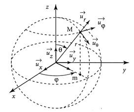
For any point M of coordinates (x0, x1, x2, x3) of Space-time, the natural base associated to point M is the set of vectors ui satisfying the following relation [GOU, Relativité Restreinte, p.492] [GOU, Relativité Générale, p.19] :
|
d(OM) = d(xi) ui |
ui thus describes the increase of the coordinate xi in the neighborhood of M (see Figure above) and is denoted vectorially : ui = d/d(xi). Not to be confused with the partial derivative operator.
Properties :
- The vectors ui constitute a vector base of Space-time.
- Each vector ui is actually a vectors field which can be written as follows :
|
In Cartesian coordinates (t, x, y, z) : ut = (1, 0, 0, 0) ux = (0, 1, 0, 0) uy = (0, 0, 1, 0) uz = (0, 0, 0, 1) The natural base is the same in every point M. In spherical coordinates (t, r, θ, φ) : ut ur = sin[θ] cos[φ] ux + sin[θ] sin[φ] uy + cos[θ] uz uθ = r cos[θ] cos[φ] ux + r cos[θ] sin[φ] uy - r sin[θ] uz uφ = -r sin[θ] sin[φ] ux + r sin[θ] cos[φ] uy The natural base changes with the point M. |
The vectors ur, uθ and uφ do not constitute an Orthonormal base of R3 for the usual Euclidean scalar product.
The associated orthonormal base (called "normalized natural base") is written : (ur, r-1 uθ, (r sin[θ])-1 uφ).
|
Proof of the ui expression in spherical coordinates : The spherical coordinates are defined from Cartesian coordinates according to the following relations (see Figure above) : x = r sin[θ] cos[φ] y = r sin[θ] sin[φ] z = r cos[θ] By using the "partial derivatives" composition law, the vector ur is written then as follows : ur = d(OM)/dr = (dx/dr) d(OM)/dx + (dy/dr) d(OM)/dy + (dz/dr) d(OM)/dz = sin[θ] cos[φ] ux + sin[θ] sin[φ] uy + cos[θ] uz Similarly we find respectively : uθ = d(OM)/dθ = (dx/dθ) d(OM)/dx + (dy/dθ) d(OM)/dy + (dz/dθ) d(OM)/dz = r cos[θ] cos[φ] ux + r cos[θ] sin[φ] uy - r sin[θ] uz uφ = d(OM)/dφ = (dx/dφ) d(OM)/dx + (dy/dφ) d(OM)/dy + (dz/dφ) d(OM)/dz = -r sin[θ] sin[φ] ux + r sin[θ] cos[φ] uy |
The Poisson equation of Newtonian gravitation (Δψ = 4 π G ρ) is a particular case of the Einstein Field Equation which corresponds to a spatially isotropic space-time, containing a non-relativistic perfect fluid (p << ρ c2), in a weak gravitational field (|ψ| << c2) and without Cosmological constant (Λ = 0).
This Newtonian limit provides the gravitational coupling coefficient (K = 8 π G c-4) used in the Einstein Field Equation as well as the Schwarzschild gravitational radius (r* = 2 G M c-2) used in the Solution of Einstein Field Equation with Schwarzschild Metric.
|
Complete proof (about the ten Einstein Field Equations) : In a weak gravitational field, we can always find a system of coordinates (xi for i = 0 to 3) = (ct, x, y, z) where the metric components are written according to the Signature convention (-, +, +, +) : (N1a) ds2 = -A2 c2dt2 + A-2 (dx2 + dy2 + dz2) (N1b) A = 1 + (ψ c-2) where ψ is the Newtonian gravitational potential (ψ = -G M/r) satisfying : |ψ| << c2 We note by o(B) the function "Small o of the quantity B in the neighborhood of 1" which is the negligible function of Landau. This metric is written at first order of ψ c-2 in the following equivalent form : (N2a) ds2 = -(1 + B + o(B2)) c2dt2 + (1 - B + o(B2)) (dx2 + dy2 + dz2) (N2b) B = 2 (ψ c-2) = -2 G M c-2 / r = B(r) Note the following useful relations : (N3a) r B,i = r dB/dxi = r (dB/dr)(dr/dxi) = -B (xi/r) = o(B) (N3b) r2 B,i,j = r2 d(B,i)/dxj = -xi r2 d(B r-2)/dxj = 3 B (xi/r) (xj/r) = o(B) (N3c) Schwartz Theorem : B,i,j = B,j,i (N3d) B,i,0 = B,0 = 0 (N3e) Laplacian operator : ΔB = ∑i[B,i,i] The gravitational potentials gij of the Metric tensor are then the following : (P1a) g00 = -(1 + B + o(B2)) = -1 + o(B) (P1b) g11 = g22 = g33 = (1 - B + o(B2)) = 1 + o(B) (P1c) gij = 0 for i and j taken different between 0 to 3 The gravitational potentials gij of the inverse Metric tensor are then as follows : gij gjk = δik where δ is the Kronecker symbol. (P2a) g00 = 1/g00 = -1 + o(B) (P2b) g11 = g22 = g33 = 1/g11 = 1 + o(B) (P2c) gij = 0 for i and j taken different between 0 and 3 Note the following useful relation : (P3) r gii,k = -r B,k + o(B2) The Christoffel symbols Γijk are then written by the relations : Γijk = Γikj = (1/2) gil (glk,j + glj,k - gjk,l) Given the relation (P2c), these relations are simplified by : (S1a) Γijk = Ki Gijk (S1b) Ki = (1/2) gii (S1c) Gijk = gik,j + gij,k - gjk,i Four distinct cases are to be considered according to the values of i, j and k. Given the relations (P3)(P2b)(P1c), these cases are written at first order of B (without term o(B2)) : Case 1 where (i = 0) and (j = 0) Examples : (ijk) = (000), (001), (010) Gijk = g0k,0 + g00,k - g0k,0 = g00,k = -B,k Γ00k = Γ0k0 = (-1/2) g00 B,k Case 2 where (i ≠ 0) and (j = i) Examples : (ijk) = (101), (110), (111) Gijk = gik,i + gii,k - gik,i = gii,k = -B,k Γiik = Γiki = (-1/2) g11 B,k Case 3 where (i ≠ j) and (j = k) Examples : (ijk) = (011), (100) Gijk = gik,k + gik,k - gkk,i = -gkk,i = B,i Γikk = (1/2) gii B,i = (1/2) g11 B,i Case 4 where (i, j and k all different) Examples : (ijk) = (012), (102) Gijk = gik,j + gij,k - gjk,i = 0 Γijk = 0 Given the relations (P2a)(P2b)(N3a)(N3b), note the following useful relations : (S2a) r Γijk = o(B) (S2b) r2 Γijk,l = o(B) (S2c) Γijk,0 = 0 The components Rij of Ricci Tensor are then written by the relations : Rij = Rkikj = (Γkij,k - Γkik,j) + (Γkkl Γlij - Γkjl Γlik) Given the relations (S2a)(S2b), these relations are simplified by : (T1) r2 Rij = r2 Rji = r2 (Γkij,k - Γkik,j) + o(B2) Hence the expression of each Rij at first order of B : Component R00 : Given relations (S2c)(N3e) and Case 3 above, we find : S1 = Γk00,k = Γ000,0 + ∑k≠0[Γk00,k] = 0 + ∑k≠0[(1/2) g11 B,k,k] = (1/2) g11 ΔB S2 = Γk0k,0 = 0 R00 = S1 - S2 = (1/2) g11 ΔB = (1/2) ΔB Component Rii for (i≠0) : Given relations (S2c)(N3e) and Cases 2, 3 and 1 above, we find : S1 = Γkii,k = Γiii,i + Γ0ii,0 + ∑k≠i, k≠0[Γkii,k] = (-1/2) g11 B,i,i + 0 + ∑k≠i, k≠0[(1/2) g11 B,k,k] = (-1/2) g11 (2 B,i,i - ΔB) S2 = Γkik,i = Γ0i0,i + ∑k≠0[Γkik,i] = (-1/2) g00 B,i,i + ∑k≠0[(-1/2) g11 B,i,i] = (-1/2) (g00 + 3 g11) B,i,i Rii for (i≠0) = S1 - S2 = (1/2) (g00 + g11) B,i,i + (1/2) g11 ΔB = (1/2) ΔB = R00 Component Rij for (i≠j) : Given the relations (S2c)(N3d)(N3c) and Cases 4, 2 and 1 above, we find : S1 = Γkij,k = S11 + S12 S11 = ∑k≠i, k≠j[Γkij,k] = 0 + 0 S12 = Γiij,i + Γjij,j Case A : If (i=0) and (j≠0) : S12 = Γ00j,0 + Γj0j,j = 0 + (-1/2) g11 B,0,j = 0 Case B : If (i≠0) and (j=0) : S12 = Γii0,i + Γ0i0,0 = (-1/2) g11 B,0,i + 0 = 0 Case C : If (i≠0) and (j≠0) : S12 = Γiij,i + Γjij,j = (-1/2) g11 B,j,i + (-1/2) g11 B,i,j = (-1/2) 2 g11 B,i,j S1 = S11 + S12 = S12 S2 = Γkik,j = S21 + S22 S21 = Γ0i0,j = (-1/2) g00 B,i,j S22 = ∑k≠0[Γkik,j] = 3 (-1/2) g11 B,i,j S2 = S21 + S22 = (-1/2) (g00 + 3 g11) B,i,j Rij for (i≠j) = S1 - S2 = Case A : 0 - (-1/2) (g00 + 3 g11) B,0,j = 0 Case B : 0 - (-1/2) (g00 + 3 g11) B,i,0 = 0 Case C : (1/2) (g00 + g11) B,i,j = 0 Rij for (i≠j) = 0 whatever Case A, B or C. The Scalar curvature is then written by the relation : R = gij Rij Given the relation (P2c), R is simplified by : (C1) R = gii Rii Hence the expression of R at first order of B : R = g00 R00 + ∑i≠0[gii Rii] = g00 R00 + g11 (3 R00) = 2 R00 = ΔB The Modified Einstein tensor is then written by the relation : Sab = Rab - (1/2) gab R + Λ gab By replacing in this relation the expressions found for gij, gij, Rij and R, we find at first order of B : E00 = R00 - (1/2) g00 R + Λ g00 = ΔB - Λ Eii for (i≠0) = Rii - (1/2) g11 R + Λ g11 = Λ Eij for (i≠j) = Rij - (1/2) gij R + Λ gij = 0 The Energy-impulse tensor of Perfect Fluid of density ρ and pressure p is then written by the relation : Tij = (c2 ρ + p) ui uj + p gij In the case of a spatially isotropic space-time containing a non-relativistic perfect fluid (p << ρ c2), then Tij is written : T00 = ρ c2 The other components Tij are all zero. The Einstein Field Equation is then written by the relation : Sab = K Tab and give at first order of B : ΔB - Λ = E00 = K T00 = K ρ c2 Λ = Eii for (i≠0) = K Tii = 0 0 = Eij for (i≠j) = K Tij = 0 Given the relation (N2b), the first equation is written : Δψ = (1/2) K ρ c4 + (1/2) Λ c2 In the case where the Cosmological constant is zero (Λ = 0), the ten Einstein Field Equations are reduced to a single equation (Δψ = (1/2) K ρ c4). By choosing a gravitational coupling coefficient K equal to : K = 8 π G c-4, we then find the Poisson equation of the Newtonian gravitation (Δψ = 4 π G ρ). By comparing the g00 of the Schwarzschild metric (g00 = -(1 - r*/r)) with the g00 of the Newtonian limit (g00 = -(1 + B)), the Schwarzschild gravitational radius is found by : r* = 2 G M c-2 |
An observer O is defined by the data of a Universe line L and a Local reference frame (e0, e1, e2, e3) along L (see Figure above) [GOU, Relativité restreinte, p.80].
The notion of observer is the cause of many misunderstandings especially on the part of philosophers. The relativistic observer does not see phenomena in the usual sense of the word 'see'. He collects position and time measurements at different points of his reference frame. This presupposes that a clock has been placed at each point of the reference frame and that this clocks set is synchronized.
An observation made by an observer O therefore consists in collecting, for an event M occurring in this reference frame, a values set for the position (x, y and z coordinates) and one for the time (t) [MAR Mécanique p.14].
If ei are the basic vectors of Space-time, the base {ei} is called orthonormal (relative to Scalar product g) when [GOU, Relativité Générale, p.26] :
|
g00 = e0.e0 = -1 gii = ei.ei = 1 for i = 1 to 3 gij = ei.ej = 0 for i and j taken different between 0 and 3 |
The matrix [gij] of this particular base, noted [ηij], is called Minkowski matrix and corresponds to the Space-time of Restricted Relativity in Cartesian coordinates.
See Convention of partial derivative.

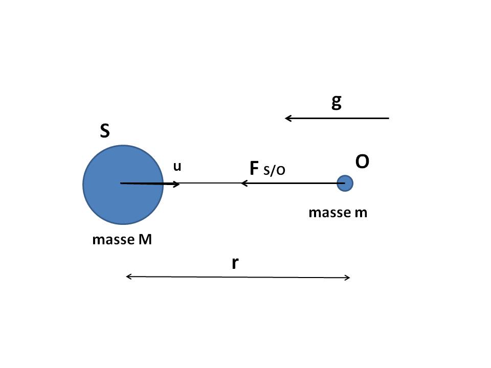
The Poisson equation was established by the French mathematician and physicist Simeon Denis Poisson.
In Newtonian universal gravitation, the (non relativistic) gravitational potential ψ is related to the density ρ by the Poisson equation :
|
Δψ = 4 π G ρ |
where Δ is the Laplacian operator (see Convention of partial derivative).
and G is the universal gravitational constant (G = 6.6726 10-11 kg-1.m3.s-2).
ψ has the dimension of m2.s-2
|
Proof : If g is the gravitational field produced at a point O of mass m by a spherical source S of mass M situated at the distance r from O (see Figure above), we have the following relations : F = m g g = -u G M / r2 g = -grad(ψ) ψ = -G M / r F = gravitational force exerted in O u = unit vector of the straight line SO The field g is otherwise characterized by the two laws : div(g) = -4 π G ρ curl(g) = -curl(grad(ψ)) = 0 in an analogous manner to the electric field E with respect to the electrical potential V without magnetic field B : div(E) = ρ_charge / ε0 curl(E) = 0 The first law (div(g) = -4 π G ρ) results from Gaussian theorem associated with the Divergence theorem as follows : Gaussian theorem : for any closed surface S with volum V and outgoing normal vector n, we have : ∑S[ g.n dS ] = -4 π G M = ∑V[ -4 π G ρ dV ] Divergence theorem : ∑S[ g.n dS ] = ∑V[ div(g) dV ] Hence the result (Poisson equation) : 4 π G ρ = -div(g) = -div(-grad(ψ)) = Δψ |
The principle of equivalence is one of the fundamental principles of General Relativity. It generalizes the Newtonian principle of equality between gravitational mass and inertial mass by asserting that a gravitational field is locally equivalent to an acceleration field.
It is stated as follows [GOU, Relativité Restreinte, p.709] : Physical measurements made by an "Inertial" Observer in a uniform gravitational field are exactly the same as those performed by a uniformly accelerated Observer.
The quadri-acceleration or 4-acceleration of any point x of Space-time is the Quadri-vector a which measures the variation of the Quadri-velocities field u along the point trajectory. This vector of dimension m-1 is defined by the following relation [GOU, Relativité Restreinte, p.38] :
|
a = (1/c) du/dτ = ai ei |
where τ is the proper Time of the point
and ei are the basic vectors of the vector space of dimension 4.
This Quadri-vector has the following properties :
a is orthogonal to u : a.u = 0
a is either a zero vector or a space-like Vector type : a.a ≥ 0
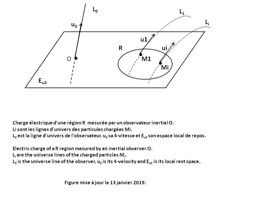
The quadri- electric power or 4- electric power is the Quadri-vector j defined by the following relation [GOU, Relativité Restreinte, p.580] :
|
Q = -∑R[ j.u0 dR ] |
Q is the total electric charge of a three-dimensional region R in the Local rest space Eu0 of an Inertial Observer O of Quadri-velocity u0. So Q represents the flow of the vector field j through R (see Figure above).
j has the dimension of a density of electric charge (in m-3.A.s).
The orthogonal decomposition of j relative to u0 is then written :
|
j = ρ u0 + c-1 J with u0.J = 0 |
ρ is the electric charge density measured by O (in m-3.A.s).
J is the electric power density measured by O (in m-2.A).
The quadri- electromagnetic potential ou 4- electromagnetic potential is the Quadri-vector A* defined by the following relation [GOU, Relativité Restreinte, p.594] :
|
Fij = d(A*j)/d(xi) - d(A*i)/d(xj) for i and j taken between 0 and 3 |
Fij is the Electromagnetic tensor.
Eu0 is the Local rest space of an Inertial Observer O of Quadri-velocity u0 (see Figure above).
In Cartesian coordinates, all components of A* are of dimension V or kg.m2.s-3.A-1
The orthogonal decomposition of A* relative to u0 is then written :
|
A* = V u0 + c A with u0.A = 0 |
V is the electric potential relative to O (in V or kg.m2.s-3.A-1).
A is the magnetic potential relative to O (in m-1.s.V or kg.m.s-2.A-1).
The quadri-force or 4-force of a material particle is the Quadri-vector f defined by the following relation [GOU, Relativité Restreinte, p.313] :
|
f = dp/dτ |
where p is the Quadri-impulse of the particle and τ its proper Time
This Quadri-vector is of dimension N or kg.m.s-2.
This Quadri-vector has the following properties :
f = d(m c u)/dτ = m c2 a + c (dm/dτ) u
f.u = -c (dm/dτ)
The quadri-impulse or 4-impulse of a simple material particle (whithout spin or internal structure) is the Quadri-vector p defined by the following relation [GOU, Relativité Générale, p.37] :
|
p = m c u |
where m is the mass at rest (or proper mass) of the particle and u is its Quadri-velocity
This Quadri-vector is of dimension kg.m.s-1 (analogous to a linear momentum).
This Quadri-vector has the following properties :
p.p = -m2 c2
See Space-time.
Figures above from left to right : Enrico Fermi and Arthur Geoffray Walker
The quadri-rotation or 4-rotation of any body of Space-time is the only Quadri-vector ω defined by the following relation [GOU, Relativité Restreinte, p.86 to 91] :
|
d(eα)/dτ = ΩFW(eα) + Ωrot(eα) ΩFW(eα) = c (a.eα) u - c (u.eα) a Ωrot(eα) = ω xu eα |
where τ is the proper Time of the body
eα are the four basic vectors of the Local reference frame linked to the body, choosing e1 tangent to the curvature a of the Universe line (condition : e1 = a/||a||)
u and a are respectively the Quadri-velocity and Quadri-acceleration of the body
"xu" is the Cross product operator between two any vectors of the Local rest space of the observer Eu, what is written : ω xu eα = Ε(u, ω, eα, .)
where :
Ε is the Levi-Civita tensor
Ε(u, ω, eα, .) is the vector representing the Linear form Ε(u, ω, eα, z) for the Scalar product g.
ω has the dimension of angular velocity (in s-1).
ΩFW is the Fermi-Walker Tensor. It affects only the components of the vectors in the plane (u, a) which is the osculating plane of the Universe line of the body.
Ωrot is the Spatial rotation Tensor. Since Ωrot(ω) = ω xu ω = 0, this tensor acts only in the subspace (of dimension 2) of the vector hyperplane Eu orthogonal to ω. In other words, Ωrot represents the spatial rotation of the trihedron (ei) in the (dimension 2) plane orthogonal to both u and ω.
This Quadri-vector has the following properties :
- ω is orthogonal to u since belonging to the vector hyperplane Eu : ω.u = 0
- ω is a space-like Vector type : ω.ω ≥ 0.
- For α = 0, we have : e0 = u, a.u = 0, u.u = -1, ω xu u = Ε(u, ω, u, .) = 0, and we find that : d(e0)/dτ = d(u)/dτ = c a
- It is proved that : ω = c T2 e1 + c T1 e3, T1 and T2 being respectively the first and the second torsion of the Universe line of the body (see Local reference frame).
See Space-time.
The quadri-velocity or 4-velocity of any point x of Space-time is the only unit Quadri-vector u which is tangent to the point trajectory and directed towards the future. This dimensionless vector is defined by the following relation [GOU, Relativité Restreinte, p.36] :
|
u = (1/c) dx/dτ = ui ei |
where τ is the proper Time of the point
and ei are the basic vectors of the vector space of dimension 4.
This Quadri-vector has the following property :
u is a unit time-like Vector : u.u = -1
Relativistic mechanics refers to mechanics compatible with the Restricted Relativity and General Relativity.
As in classic mechanics, the subject can be divided into two : the kinematics that describes the movement in terms of Quadri-position, Quadri-velocity, Quadri-rotation and Quadri-acceleration, and the dynamics that describes the movement cause in terms of Quadri-impulse, Angular momentum, Quadri-force and Energy.
In addition, when there is a change of Observer, some quantities are transformed : lengths and durations (Lorentz-Poincaré transformation), velocities [GOU, Relativité restreinte, p.141], accelerations [GOU, Relativité restreinte, p.151], frequencies (Doppler effect), angles of observation (Aberration) and images (Image).
If (ds) is the distance (or interval) between two events infinitely close to the Space-time, then the Relativistic metric is the "square" of this distance and is written :
|
ds2 = gij dxi dxj |
In the curved Space-time of General Relativity, this metric can be negative, zero or positive, and is written in Cartesian coordinates :
ds2 = g00 (c dt)2 + g01 (c dt) dx + g02 (c dt) dy + g03 (c dt) dz +
g10 dx (c dt) + g11 dx2 + g12 dx dy + g13 dx dz +
g20 dy (c dt) + g21 dy dx + g22 dy2 + g23 dy dz +
g30 dz (c dt) + g31 dz dx + g32 dz dy + g33 dz2
The coefficients gij are the components of the Metric tensor.
Note that the quantity ds2 is always negative for a non-zero mass particle, the vector tangent to its Universe Line being a time-like Vector.
The Ricci tensor (Rab) is a Symmetric Tensor of order 2 producted by Contraction of the Curvature tensor. It is therefore a Tensor that measures the local deformation of Space-time but incompletely.
According to the Classic Sign Conventions (MTW) it is producted by Contraction of the Curvature tensor on the first and third index. Using the Convention of partial derivative, its components are the following :
|
Rij = Rkikj = Γkij,k - Γkik,j + Γkkl Γlij - Γkjl Γlik |
where Γijk are the Christoffel symbols.
In Cartesian coordinates, all the components are of dimension m-2
Warning : the Ricci tensor can be zero without the Curvature tensor being it.
Warning : Unlike classic MTW sign conventions, some authors contract the Tensor of curvature on the first and fourth indexes, which amounts to defining the opposite of the Tensor of Ricci.
The scalar curvature of Space-time is a number (R) of dimension m-2 producted by Contraction of the Ricci tensor in the form :
|
R = gij Rij = Rii |
R is actually the trace of the Ricci tensor.
Scalar product of two vectors :
Using the Convention of summation, the scalar product of two arbitrary vectors x and y is written :
|
x.y = gij xi yj = xi yi = xi yi = gij xi yj |
where the coefficients gij are the components of the Metric tensor.
Some authors also use the following two notations :
x.y = <x, y> = g(x, y)
|
Proof : x.y = (xi ei).(yj ej) = (ei.ej) xi yi = gij xi yj |
The norm ||x|| of any vector x is the square root of the absolute value of the scalar product of x by itself :
||x|| = (|x.x|)1/2
Scalar product of two Tensors U and V of order 2 :
T = Uij.Vkl of component : T = Uij Vij
T = Uij.Vkl of component : T = gik gjl Uij Vkl
T = Uij.Vkl of component : T = gik gjl Uij Vkl
The metric of Karl Schwarzschild is a Relativistic metric corresponding to the static gravitational field with central symmetry. This is the case of the Sun and many stars. The central body is spherically symmetrical and not necessarily static (for example, a pulsating star that oscillates radially or a star that collapses into a Black hole while maintaining its spherical symmetry). The gravitational field must be static even if it is not static in the area where the matter is located. Note that the gravitational field is necessarily static in spherical symmetry and in vacuum (Birkhoff theorem).
In spherical coordinates (r > 0, colatitude θ = [0, π], longitude φ = [0, 2 π]) (see Figure in Space-time), the metric is written as follows for any coordinate system (ct, r, θ, φ) and by taking the Signature convention (-, +, +, +) :
|
ds2 = -e2 μ c2dt2 + e2 α dr2 + r2 dθ2 + r2 sin2[θ] dφ2 |
where μ and α are only functions of r.
The gravitational potentials gij then are the following :
|
g00 = -e2 μ ; g11 = e2 α ; g22 = r2 ; g33 = r2 sin2[θ] ; gij = 0 for i and j taken different between 0 and 3 with (see Solution of Einstein Field Equation with Schwarzschild metric) : g00 = -(1 - r*/r) g11 = 1/(1 - r*/r) where r* is the Schwarzschild radius. |
|
Proof of metric ds2 [GOU, Relativité Générale, p.116] : The spherical center symmetry of the field allows to write the metric in the following form : ds2 = -N2 c2dt2 + A2dr2 + B2 (dθ2 + sin2[θ] dφ2) where the components N, A and B are functions of r and t. The staticity of the field then allows to delete the dependence of t in these components. The coordinate r can be otherwise choosen as the areolar radius of the invariance spheres related to the spherical symmetry. This is written : N(r,t) = N(r) = eμ A(r,t) = A(r) = eα B(r,t) = B(r) = r |
The Shapiro effect manifests itself as a delay of any electromagnetic signal (including light) near a gravitational field, compared to the propagation time that this signal would have in flat space-time.
This phenomenon was predicted in 1964 by Irwin Shapiro and detected in 1966 and 1967 by the Haystack radar antenna at MIT (Massachusetts Institute of Technology).
The (-, +, +, +) signature of the Metric tensor, called Lorentzian signature, means that there exists a basis of the vector space E such that the Scalar product g(u,v) is expressed as a function of the components ui and vj of the vectors u and v in the following form [GOU, Relativité Restreinte, p.8] :
g(u,v) = -u0v0 + u1v1 + u2v2 + u3v3
Warning : Unlike classic MTW sign conventions, some authors use the (+, -, -, -) signature instead of (-, +, +, +), which amounts to using -g instead of g.
The classic convention (-, +, +, +) has the advantage of not distinguishing between Quadri-vectors and tri-vectors because the Scalar product induced by g on the space-like hyperplanes (three-dimensional cuts of Space-time at t = constant) coincides with the Euclidean scalar product of three-dimensional space.
In Restricted Relativity, it is shown that two events located in different places can be simultaneous in one reference frame without being in another. The notion of simultaneity loses its universal character.
|
Proof : Let two simultaneous events (x1, y1, z1, t1) and (x2, y2, z2, t2 = t1) be in the referential frame R. In the reference frame R' in uniform rectilinear translation with respect to R, the duration (t'2 - t'1) between these two same events is written given the Lorentz-Poincaré transformation : t'2 - t'1 = γ ( (t2 - t1) - B (x2 - x1) ) = -γ B (x2 - x1) γ and B being given by equations (L3) ans (L4). When the two events are not located at the same points, the spatial difference (x2 - x1) in R is not zero. The temporal difference (t'2 - t'1) in R' is therefore not zero despite the simultaneity (t2 = t1) of the two events in R. |
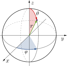
Space-time is a four-dimensional space where time is no longer a separate quantity independent of space but a variable playing the same role as spatial variables. The notion of Simultaneity is no longer universal.
Definition [GOU, Relativité Restreinte, p.24] :
Space-time (called Minkowski space-time) is defined by the set of four mathematical objects :
- Real affine space of dimension 4, associated with a oriented vector space E (depending on whether the base is Direct or indirect)
- Scalar product of (-, +, +, +) Signature, associated with the Metric tensor g
- Light-cone with its two time arrows (past sheet and future sheet)
- Levi-Civita tensor E associated with the metric g
Quadri-vector and coordinates :
In this space-time of origin O fixed, a point or event x(x, y, z, t) is identified by a four-dimensional vector x called Quadri-vector or 4-vector whose components are denoted :
|
- In Cartesian coordinates : x0 = ct ; x1 = x ; x2 = y ; x3 = z - In spherical coordinates (r > 0, colatitude θ = [0, π], longitude φ = [0, 2 π]) : x0 = ct ; x1 = r ; x2 = θ ; x3 = φ |
The spherical coordinates are defined from Cartesian coordinates according to the following relations (see Figure above) [GOU, Relativité Générale, p.20] :
|
x = r sin[θ] cos[φ] y = r sin[θ] sin[φ] z = r cos[θ] |
From a geometrical view point, r gives the area (A = 4 π r2) of the invariance spheres related to the spherical symmetry (spheres with t = constant and r = constant). The coordinate r is sometimes called areolar radius [GOU, Relativité Générale, p.59].
Physical meaning :
The coordinates ct, x, y, z, r, θ and φ have no physical meaning (measurable directly) [GOU, Relativité Générale, p.59] [GOU, Relativité Restreinte, p.430] [EIS Lumière, p.7]. They are only a formal means of labeling the points of space-time.
Only the conclusions, accessible by the elimination of the coordinates, have an objective meaning.
Only the Proper Time has a physical meaning in Restricted and General Relativity, and the distances are measured in Proper time on Geodesic trajectories [EIS Lumière, pp 7-8].
Flat space-time :
Space-time is flat (Curvature tensor identically zero) only if it is Minkowski space-time [GOU, Relativité générale, p.200].
The space-time structure constant is a constant that is similar to a limiting speed of propagation of interactions. It appears during the demonstration of the equations of the Lorentz-Poincaré Transformation and corresponds to the causality postulate that guarantees the temporal order of causal events in all inertial reference frames.
This constant is taken equal to the highest speed currently measured which is that of electromagnetic phenomena in a vacuum, in this case the speed of light in a vacuum (c).
The cosmological model that best describes the History and behavior of the observable universe is the standard model of cosmology (or Big Bang model or Λ-CDM model meaning "Λ Cold Dark Matter").
This model represents an universe with the following properties (see curve C4 in Figure above) :
1. Model with Big Bang (such that the scale factor a(t) tends towards 0 when t tends towards 0).
2. Spatially homogeneous and isotropic on a large scale (thus also with constant spatial curvature). See Friedmann-Lemaitre-Robertson-Walker metric
3. Whose spatial curvature is zero (k = 0). Not to be confused with the curvature of space-time (Ricci tensor) which measures the spatio-temporal deformation of the universe.
4. Filled with a perfect fluid (galaxy gas) of density ρ and equation of state w = p/(ρ c2) which models matter and energy in the universe. This fluid is made up of several components :
4.1. Ordinary matter consisting of protons, neutrons and electrons forming atoms and molecules. It is a cold, baryonic and non-relativistic matter (w = 0).
4.2. Dark matter which is cold, non-baryonic and non-relativistic (w = 0).
4.3. Radiation and hot matter including all forms of electromagnetic radiation (photons) and relativistic particles such as neutrinos. This component is hot and relativistic (w = 1/3).
4.4. Dark Energy (w = -1) requiring : Λ > 0
5. Consistent with the Standard Model of Particle Physics.
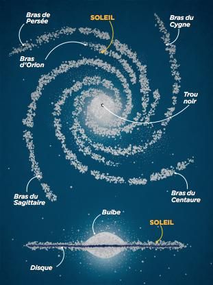
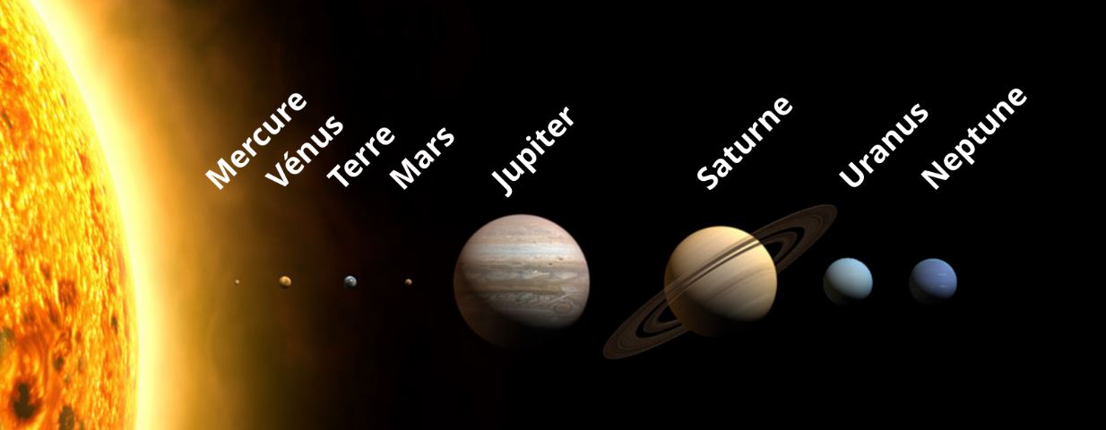
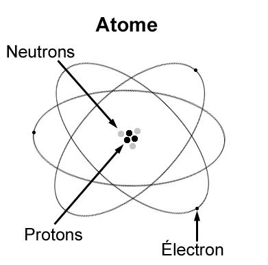
Figures : left (Milky Way with our Sun), middle (our Solar system), right (Atom).
The standard model of particle physics populating the universe is as follows, with a description presented in hierarchical form.
1.
Forces of the universe :
Four types of forces govern the universe :
- Strong force : Force acting on Quarks (cohesion of Hadrons) and Nucleons (cohesion of the atomic Nucleus). Short range : 10-15 m. Mediators : Gluons for the interaction between Quarks and Mesons for the interaction between Nucleons.
- Electromagnetic force : Force acting on electrically charged particles (Electrons, Protons, Ions, Quarks, etc.). Infinite range, the intensity of which decreases with distance r according to the 1/r2 law. Mediators : Photons.
- Weak force : Force acting on Quarks and Leptons, responsible for certain types of radioactive decay and nuclear reactions in stars. Short range : 10-18 m. Mediators : W and Z Bosons.
- Gravitational force : Force acting on all particles with energy, quantum or not, massive or not. Infinite range but extremely weak in intensity compared to the other three forces (and negligible in quantum physics). Hypothetical mediator : Graviton.
Some forces are subject to unification :
- Electroweak model (Weinberg, Salam, Glashow, 1960) unifies the weak and electromagnetic forces.
- Grand Unified Theories (GUT) seek to unify the strong force with the already unified electroweak force.
- Theory of Everything seeks to unify the gravitational force with the other three forces.
2.
Astronomical description :
Observable universe = Superclusters + Galactic filaments + Cosmic voids. Size = about 93 billion light-years.
| Superclusters = set of Galactic clusters. Size = about 500 million light-years. Example : Laniakea Supercluster which includes the Virgo Cluster and the Local Group.
| | Galactic cluster = set of Galaxies. Size = about 10 million light-years. Examples : Virgo Cluster which contains more than a thousand Galaxies ; the Local Group which contains about 50 Galaxies including the Milky Way and Andromeda.
| | | Galaxy = Stars + Planetary systems + Gas and dust. Size = about 100 000 light-years. Example : the Milky Way which contains more than 100 billion Stars including our Sun.
| | | | Star = celestial body composed of Gas in nuclear fusion. Example : our Sun.
| | | | Planetary system = set of planets, moons and other bodies orbiting a Star. Size = about 0.002 light-years or 20 billion km. Example : our Solar System which includes Earth, Mars, Jupiter, etc.
| | | | Gas and dust = diffuse constituents in Galaxies. Example : clouds of gas and dust contained in the Orion Nebula.
| Galactic filament = filament of Dark Matter and Gas, channeling Matter and Energy between Superclusters and Galactic Clusters. Size = about 1 billion light years. Example : the Great Wall of Hercules-Corona Borealis (HCB Great Wall).
| Cosmic void = region almost empty of matter. Size = about 100 million light years. Example : the Boötes Void is located in the constellation Boötes, near the Hercules Supercluster.
The relative movements are as follows :
| On a planetary scale : proper rotation of moons and artificial satellites + orbital motion around the planets
| On a stellar scale : proper rotation of planets and other bodies + orbital motion around the Stars
| On a galactic scale : proper rotation of the Stars + orbital motion around the galactic center + vertical oscillation relative to the galactic plane (epicyclic oscillation)
| On an intergalactic scale : proper motion of the Galaxies
| On a cosmological scale : expansion of the universe
3.
Physical description :
Nota : isolated words (without commentary) are defined in the Basic Vocabulary.
Observable universe = Matter + Energy
| Matter = Ordinary Matter + Non-ordinary Matter
| | Ordinary (or baryonic) Matter = Molecules (which can exist as solid, liquid, gas or plasma; example water (H2O)) + isolated Atoms (example: Helium (He)) + Anti-particles
| | | Molecule
| | | Atom
| | | Anti-particles
| | Non-ordinary Matter = Quarks + Non-ordinary Leptons + Electronic Neutrinos + Bosons + Anti-particles + Dark Matter
| | | Quark
| | | Non-ordinary Lepton
| | | Electronic Neutrino
| | | Boson
| | | Anti-particles
| | | Dark matter = hypothetical matter producing excess gravity that Galaxies need to keep themselves from breaking apart during their rotation
| Energy = Electromagnetic radiation + Cosmic radiation + Dark energy
| | Electromagnetic radiation = energy carried by Photons, classified by frequency or wavelength = Gamma rays + X-rays + Ultraviolet + Visible light + Infrared + Microwaves + Radio waves
| | | Gamma rays = very high energy produced during nuclear and astrophysical phenomena
| | | X-rays = used in medical imaging
| | | Ultraviolet = responsible for sunburn and chemical reactions in the upper atmosphere
| | | Visible light = what the human eye can see
| | | Infrared = heat emitted by objects
| | | Microwaves = used to heat food
| | | Radio waves = low energy used for long-distance communication
| | Cosmic radiation = energy carried by high-energy particles (often Helium Protons) from cosmic sources such as supernovae and active galactic nuclei
| | Dark energy = hypothetical energy that tends to accelerate the expansion of the universe
4.
Basic vocabulary :
Molecule = set of grouped Atoms, held by chemical bonds.
Atom = Nucleus + Electrons
| Nucleus (or nucleons) = Protons + Neutrons
| | Proton = positively charged particle (spin = 1/2) = two "up" Quarks and one "down" Quark, held by the strong force
| | Neutron = uncharged particle (spin = 1/2) = two "down" Quarks and one "up" Quark, held by the strong force
| Electron
Anti-particle = particle with the same mass and spin as the corresponding particle, but with opposite additive quantum numbers.
The Anti-particles can be Elementary (examples : Anti-quark, Anti-electron, Anti-muon, Anti-tau, Anti-neutrino, Anti-boson) or Composite (examples : Anti-proton, Anti-neutron, Anti-Nucleus, Anti-atom).
Some particles, called "self-conjugated", are their own Anti-particle (examples : Photon, Z Boson, Neutral Pion).
Fermions = particles that constitute matter. They obey the Pauli exclusion principle according to Fermi-Dirac statistics and have a semi-integer spin (1/2, 3/2, 5/2, etc.) which does not allow them to simultaneously occupy the same Quantum state.
| Composite Fermion = any assembly of Elementary Fermions giving a composite particle of semi-integer spin
| Elementary Fermion = any Fermion of Quark or Lepton type (spin = 1/2)
| | Quark = smallest particle in the Standard Model of particle physics, affected by the strong force, characterized by spin 1/2 and six "flavors" : Up, Charm and Top/Thruh (charge = +2/3), Down, Strange and Bottom/Beauty (charge = -1/3)
| | Lepton = all spin 1/2 particle, not affected by the strong force = Electron + Muon + Tau + Neutrino
| | | Electron = particle orbiting the Nucleus, negatively charged (spin = 1/2). Does not contain Quarks.
| | | Muon = negatively charged particle (spin = 1/2)
| | | Tau = extremely short-lived, negatively charged particle (spin = 1/2)
| | | Neutrino = extremely low-mass, uncharged particle (spin = 1/2), characterized by three "flavors" : electronic, muonic and tauic
| | Ordinary Leptos = stable Leptos = Electron + electronic Neutrino
| | Non-ordinary Leptos = unstable Leptos that decay rapidly = Muon + Tau + muonic Neutrino + tauic Neutrino
Bosons = particles that carry the fundamental forces = Gauge Bosons + Higgs Boson
| Gauge bosons = particles that transmit the fundamental forces = Photons + Gluons + W and Z bosons + Gravitons. They obey the superposition principle according to Bose-Einstein statistics and have an integer spin (0, 1, 2, etc.) allowing them to simultaneously occupy the same Quantum state.
| | Photon = massless, uncharged particle, spin = 1, mediator of the electromagnetic force.
| | Gluon = massless, uncharged particle, spin = 1, mediator of the interaction between Quarks in the strong force.
| | W and Z bosons = three massive particles (W+, W- and Z), charged for W+ and W-, uncharged for Z, spin = 1, mediator of the weak force.
| | Graviton = hypothetical, uncharged particle, spin = 2, mediator of the gravitational force.
| Higgs boson = uncharged particle, spin = 0, associated with the Higgs field that acts on other Elementary particles, giving them a form of potential energy perceived as their mass.
Elementary particles = Elementary Fermions + Bosons + Elementary Anti-particles
Composite particles = Molecules + Nuclei + Composite Fermions + Ions + Hadrons
| Molecule
| Nuclei
| Composite Fermion
| Ion = Atom or Molecule electrically modified, having lost Electrons (Cation) or gained Electrons (Anion). Examples: Sodium Ion (NA+) having lost an Electron, Chloride Ion (Cl-) having gained an Electron.
| Hadron = any particle containing Quarks, Anti-quarks and Gluons = Baryon + Meson + Exotic Hadron
| | Baryon = particle composed of three Quarks (examples : Proton, Neutron)
| | Meson = particle composed of a Quark and an Anti-quark (examples : pi Meson (Pion), K Meson (Kaon)), mediator of the interaction between Nucleons in the strong force.
| | Exotic Hadron = any other combination of Quarks and Anti-quarks (examples : tetraquark, pentaquark)
Relativistic particles = particles whose speed is close to that of light, therefore subject to the laws of Relativity = Electrons + Photons + Gluons + Neutrinos
5. Characterization of particles :
See Quantum physics.
6. Characterization of a galaxy :
A galaxy is characterized mainly by the following list of characteristics.
Example of the Milky Way :
| Age = 13 billion years (formed 800 million years after the Big Bang)
| Formation = Initial formation of a "thick disk", then collision and merger, two billion years later, with a dwarf galaxy called "Gaia-Enceladus".
| Lifespan = Expected collision in 4.5 billion years with the Andromeda galaxy, with the two galaxies merging for another two to three billion years.
| Type = Barred spiral galaxy S(B)bc I-II
| Mass = about 2.0 1011 solar masses
| Dimensions = Disk with a diameter of 150,000 light years and a thickness of 6,000 light years
| General composition (from the center to the periphery) = 1. Very dense central bulge around the galactic center, 2. Galactic disk structured in spiral arms containing the majority of Stars, especially young Stars, 3. Galactic halo containing globular clusters (old Stars) as well as a large quantity of Dark Matter.
| Composition of central bulge (from the center to the periphery) = 1a. Super-massive black hole ("Sagittarius A*") located at the heart of the galaxy, 1b. "Nuclear Star Cluster" composed mainly of old Stars, 1c. "Sagittarius A West", mini-spiral structured in filaments of hot ionized gas, 1d. "Sagittarius A East", remnants of a supernova after its explosion, 1e. Circumnuclear disk (torus of cold gas and dust).
| Composition of the galactic disk (observed from the Galactic North Pole) = several spiral arms whose winding is counterclockwise. The order of the arms, from the outside to the inside of the galaxy, is as follows (but without scientific consensus) : 1. Perseus, 2. Cygnus (or Eagle), 3. Norma, 4. Sagittarius (or Sagittarius-Carina), 5. Centaurus (or Scutum-Centaurus), 6. Orion (or Local) in which our Solar System is located.
| Motion relative to the cosmological frame of reference :
| | Proper rotation = maximum in the galactic disk (including at the level of our Sun) with a tangential speed of about 250 km/s
| | Speed of movement = 600 km/s relative to the cosmic background and 110 km/s in the direction of the Andromeda galaxy (approach)
| Particularities :
| | Appearance = the Milky Way is visible as a milky band in the night sky, hence its name.
7. Characterization of a star :
A Star is characterized mainly by the following list of characteristics.
Example of our Sun :
| Age = 4.57 billion years
| Formation : A gravitational collapse of a dense region of a vast cloud of gas and dust, called "solar nebula", triggered nuclear reactions at its center, marking the birth of our Sun.
| Lifespan : In five billion years, the Sun will begin to transform into a red giant, a phase that will last a few hundred million years. Then, the Sun will become a white dwarf, surrounded by a planetary nebula resulting from the ejection of its outer layers.
| Mass = 1.989 1030 kg
| Equatorial radius = 696,000 km
| Average density = 1.408 103 kg/m3
| Internal composition = Hydrogen (73 %) + Helium (25 %) + metals (2 %)
| Radiated power (or intrinsic luminosity L) = 3.8 1026 W
| Surface temperature = 5500 C
| Surface gravity = 274 m/s2
| Position of the rotation axis relative to the perpendicular to the galactic plane = 23 to 30 in inclination
| Proper rotation period = between 25 days (equator) and 36 days (poles)
| Orbit relative to the galactic center (Milky Way) :
| | Average distance to the galactic center = 26,000 light years
| | Period of revolution = 225 to 250 million years
| | Position of the Sun relative to the galactic plane = approximately 48 light years above the galactic plane in the direction of Galactic North
| | Orbital inclination relative to the galactic plane = 7
| | Average orbital speed = 220 km/s
| Particularities :
| | Presence of Planetary system = Yes (our Solar system)
| | Presence of natural satellites = No
| | Presence of rings = No
| | Magnetic field = Yes (5000 μT on the surface, inclined by about 10 relative to the axis of rotation)
8. Characterization of a planet :
A planet is a celestial body that revolves around a star, has a spherical shape, and has cleared its orbit of any independent body of comparable size, with the exception of its possible natural satellites (moons). This cleaning consists of driving out intruders (ejection), merging with them (accretion) or orbiting them (satellization).
Thus Pluto, although spherical and orbiting the Sun, is not a planet but a so-called "dwarf planet" because it shares its orbital region with many small independent bodies.
All other celestial bodies that orbit a star, without being a planet, dwarf planet, or natural satellite, are called "small bodies" and primarily include asteroids and comets.
A planet is characterized mainly by the following list of characteristics.
Example of the Earth :
| Age = 4.54 billion years
| Formation : Collisions between dust and gas particles in the protoplanetary disk surrounding our young Sun gradually created increasingly massive aggregates, leading to the formation of the planet.
| Lifespan : In one billion years, Earth will lose all of its water due to a 10 % increase in the Sun's luminosity, making life impossible for most life forms. Four billion years later, it will lose its atmosphere when the Sun becomes a red giant, making the planet inhospitable.
| Mass = 5.972 1024 kg
| Equatorial radius = 6,371 km
| Average density = 5.515 103 kg/m3
| Internal composition = solid inner core, liquid outer core, mantle, crust
| Atmospheric composition = 78 % nitrogen, 21 % oxygen, traces of carbon dioxide (0.04 %), water vapor, argon, etc.
| Atmospheric pressure at sea level = 101.3 kPa = 1 atm
| Surface temperature (in the shade) = between -89 C (Vostok station in Antarctica) and +57 C (Death Valley in California, USA), with an average global temperature of 14 C
| Surface gravity = 9.807 m/s2
| Position of the rotation axis relative to the perpendicular to the ecliptic = 23.44 in inclination, and almost constant in orientation
| Proper rotation period (sidereal day) = 23 h 56 min 4 s
| Orbit relative to the Sun :
| | Average distance from the Sun (semi-major axis d) = 149.6 106 km
| | Perihelion (point closest to the Sun, early January) = 147.1 106 km
| | Aphelion (point furthest from the Sun, early July) = 152.1 106 km
| | Period of revolution = 365.256 days
| | Eccentricity of the orbit = 0.0167
| | Orbital inclination relative to the plane of the ecliptic = 0 by definition
| | Average orbital speed = 29.78 km/s
| | Apparent brightness of the Sun from Earth (or illuminance E = L / (4 π d2)) = 1360 W/m2
| Special features :
| | Position of the ecliptic relative to the galactic plane (principal plane of the Milky Way) = 60 in inclination, and according to two opposite points in intersection
| | Presence of natural satellites = Yes (The Moon)
| | Presence of rings = No
| | Magnetic field = Yes (25 to 65 μT at the surface, inclined about 11 to the rotation axis)
| | Albedo = variable depending on the surface (oceans, continents, ice)
| | Presence of life = Yes
9. Characterization of a natural satellite :
A natural satellite (or moon) is a celestial body that revolves around another celestial body other than a star, generally a planet or an asteroid.
It is characterized mainly by the following list of characteristics.
Example of the Moon :
| Age = 4.51 billion years
| Formation (large impact hypothesis) : The Moon is believed to have formed from debris resulting from a massive collision between the young Earth and a Mars-sized planetary body called "Theia".
| Lifespan : The Moon is now considered geologically dead. In five billion years, the transformation of the Sun into a red giant will accentuate its dead and inhospitable state.
| Mass = 7.347 1022 kg
| Equatorial radius = 1737 km
| Average density = 3.34 103 kg/m3
| Internal composition = core, mantle, crust
| Atmospheric composition (exosphere) = 25 % neon, 25 % helium, 23 % hydrogen, 20 % argon, traces of sodium and oxygen
| Atmospheric pressure at the surface = extremely low (about 10-13 Pa)
| Surface temperature = between -173 C (lunar night) and +127 C (lunar day)
| Surface gravity = 1.62 m/s2
| Position of the axis of rotation relative to the perpendicular to its orbital plane = 1.5 in inclination, and almost constant in orientation
| Proper rotation period = 27.32 days
| Orbit relative to the Earth :
| | Average distance to the Earth = 384,400 km
| | Perigee (closest point to the Earth) = 363,300 km
| | Apogee (furthest point from the Earth) = 405,500 km
| | Period of revolution = 27.32 days (identical to the proper rotation period)
| | This phenomenon of gravitational locking is mainly due to the difference in gravitational attraction exerted by the Earth on the parts of the Moon that are closer and more distant, creating a torque of forces tending to align its own rotation with its orbital revolution.
This phenomenon would have occurred even if the Earth had no oceans. It is independent of the terrestrial tides that influence the long-term evolution of the lunar orbit and the Earth's rotation, without any impact on the synchronous rotation of the Moon.
| | Eccentricity of the orbit = 0.0549
| | Orbital inclination relative to the plane of the ecliptic = 5.14
| | Average orbital speed = 0.283 km/s
| Special features :
| | Presence of rings = No
| | Magnetic field = No
| | Albedo = Yes
| | Presence of life = No
The most common standard times are :
- Greenwich Mean Time (GMT) is the time on the meridian of Greenwich in England (0 longitude). The term "Mean" refers to the fact that noon GMT is the time on average each year when the Sun culminates at the Greenwich meridian. This time which is relatively imprecise because linked to the rotational speed variation of the Earth and to the ellipticity of its orbit, was used until 1972.
- Universal Time (UT) replaces the Greenwich Mean Time (GMT) with a difference because the GMT was calculated on noon and the UT on midnight.
- Terrestrial Time (TT) is the time of a observer fixed on the Earth surface. TT takes relativistic effects into account (Einstein effect in General Relativity and durations dilation in Restricted Relativity). TT is given by the following Relativistic metric [GOU, Relativité Générale, p.207] :
d(TT) = c-1 (-gij dxi dxj)1/2
where :
gij = components of the Metric tensor near the Earth (with weak gravitational field ψ)
xi = coordinates of the observer in the Space-time of GCRS celestial reference frame (with t = GCT)
The Earth (with REarth = 6378 km) rotating around the axis θ = 0 at the angular velocity dφ/dt = ΩEarth = 2 π / (23 h 56 mn) = 7.29 10-5 rad.s-1, the coordinates xi of an observer of colatitude θ0 are :
x0 = ct
x1 = r0
x2 = θ0
x3 = φ0 + ΩEarth t
TT time differs from GCT time only by a constant factor independent of the position on Earth [GOU, Relativité Générale, p.208] :
d(TT) = (1 + c-2 U0) dt
U(r, θ, φ) = ψ(r, θ, φ) - (1/2) ( ΩEarth r sin[θ] )2
U0 = U(r0 = REarth, θ0 = π/2, φ0) = -6.969 10-10 c2
- International Atomic Time (IAT) is calculated from the comparison of the Terrestrial Times of about 300 atomic clocks in the world. IAT is under the responsibility of the International Bureau of Weights and Measures (IBWM).
- Universal Time Coordinated (UTC) (or Zulu Time or Z Time) differs from IAT by an integer number of seconds, currently 37 since 1972, so as to be true to the UT time within less than 0.9 second. These leap seconds are added at the initiative of the International Earth Rotation and Reference Systems Service (IERS) to ensure that, on average over the years, the Sun culminates at the Greenwich meridian at 12:00:00 UTC to within 0.9 second.
See Convention of summation (called "Einstein convention").
A Tensor is usually neither symmetrical nor antisymmetric.
Tensor of order 2
A Tensor Tab is said to be symmetrical when : Tab = Tba
A Tensor Tab is said to be antisymmetrical when : Tab = -Tba
Any Tensor Tab can be expressed as sum of a symmmetrical Tensor Sab and an antisymmetrical Tensor Aab such as :
Sab = (1/2)(Tab + Tba)
Aab = (1/2)(Tab - Tba)
Tensor of order greater than 2
A Tensor is said to be symmetric (resp. antisymmetric) with respect to a pair of indexes of the same variance (i.e. all covariants ou contravariants) if the permutation of these indexes keeps (resp. changes to its opposite) each component of the Tensor.
The Tensor is said to be completely symmetric (resp. completely antisymmetric) if it is symmetric (resp. antisymmetric) with respect to any pair of indexes of the same variance.
Examples for Tensor Tklmij :
- if Tklmij = Tkmlij, then it is symmetric with respect to l and m.
- if Tklmij = Tklmji, then it is symmetric with respect to i and j.
- if Tklmij = -Tkmlij, then it is antisymmetric with respect to l and m.
- if Tklmij = -Tklmji, then it is antisymmetric with respect to i and j.
- if Tklmij = Tkmlij = Tmlkij = Tlkmij, then it is completely symmetrical with respect to its contravariant indexes.
- if Tklmij = -Tkmlij = -Tmlkij = -Tlkmij, then it is completely antisymmetrical with respect to its contravariant indexes.
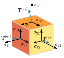
The term "tensor" was introduced by the physicist Woldemar Voigt to represent mathematically the tensions in a solid (see Figure above).
Pragmatic definition :
The concept of tensor is a generalization of the notion of vector as a mathematical object invariant by base change.
A tensor is a multilinear function of the coordinates of space, defined in an n-dimensional vector space by nm components where m is the order of the tensor.
The tensor of order 0 is a scalar (number independent of the chosen base) and has a single component.
The tensor of order 1 is a vector with n components. Note that, during a base change, the components of a vector change while the vector itself does not change.
The tensor of order 2 is a square matrix with n2 components which satisfies any one of the criteria of Tensoriality.
The tensor of order 3 is a cubic matrix with n3 components which satisfies any one of the criteria of Tensoriality.
Each tensor also has a valence or type denoted (p, q) where p is the number of contravariant index (indicated in the upper position) and q the number of Covariant index (indicated in the lower position) according to : m = p + q.
For any tensor T, its components can be contravariant (example : Tijk), covariant (example : Tijk) or mixed (example : Tijk is a mixed tensor of order 3 with one contravariant index i and two covariant indexes j and k).
The tensorial calculation has the advantage of being freed from all systems of coordinates and the results of the mathematical developments are thus invariant by change of reference frame (see Covariance of physical law).
Mathematical definition [GOU, Relativité Restreinte, p.472 and 21] :
A tensor (T) is a multilinear application of a vector Space (E) and its Dual space (E*) to the field (R) of real numbers.
If ω1, ... ,ωp and v1, ... ,vq denote respectively any Linear forms ω of Dual space E* and any vectors v of space E (of dimension n), then any tensor of type (p, q) is an application T(ω1, ... ,ωp, v1, ... ,vq) of E*p x Eq to R, which is linear with respect to each of its m arguments (m = p + q).
For any scalar λ and argument a, we have the following identities :
|
T(ω1, ... ,λ a + a', ... ,vq) = λ T(ω1, ... ,a , ... ,vq) + T(ω1, ... ,a', ... ,vq) |
In old books, a tensor is defined not as a multilinear application, but as an array of "numbers" T i1... ip j1... jq which transforms according to the general transformation law by Base change.
Tensor examples :
- Simple example in a vector space E of dimension 3 (operators . and x denoting respectively scalar product and cross product) :
The T application that matches the vector triplet (u, v, w) to the scalar : 5 u.(v x 2 w) is a tensor of order 3.
The A application that matches the vector triplet (u, v, w) to the scalar : 5 u.(v + 2 w) is not a tensor. It is not linear with respect to its second and third arguments.
- Any scalar s is a tensor of type (0, 0).
- Any vector v is a tensor of type (1, 0).
- Any Linear form ω is a tensor of type (0, 1).
- The Metric tensor g and the Electromagnetic tensor F are tensors of type (0, 2).
- The Curvature tensor Rijkl is a tensor of type (1, 3).
- The Levi-Civita tensor Ε is a tensor of type (0, 4).
Tensor components [GOU, Relativité Restreinte, p.474, 475] :
Because of multilinearity of T, the np + q components of T are written as a function of the vectors of the base {ej} and elements of the Dual base {ei} as follows :
|
T i1... ip j1... jq = T(ei1, ... ,eip, ej1, ... ,ejq) and we have the following general relation : T(ω1, ... ,ωp, v1, ... ,vq) = T i1... ip j1... jq (ω1)i1... (ωp)ip (v1)j1... (vq)jq |
The tensor product of two Tensors of order m and n allows to form a Tensor of order (m + n) which "groups" the two Tensors.
The resulting Tensor Tijkl of the tensor product Uij ⊗ Vkl thus has as components : Tijkl = Uij Vkl
The tensor product preserves the nature (covariant or contravariant) of each index of the original tensors.
The tensor product is associative (U ⊗ (V ⊗ W) = (U ⊗ V) ⊗ W) (cf [GOU, Relativité restreinte, p.473]), noncommutative and distributive with respect to the Tensor addition (U ⊗ (V + W) = U ⊗ V + U ⊗ W)
Any mathematical object that satisfies one of the following tensorial criteria is a Tensor.
Criterion 1 : any object defined intrinsically as a multilinear form (see Tensor).
Criterion 2 : any numbers table that transforms by Base change according to the general transformation law.
Criterion 3 : any result of an elementary operation or a combination of Elementary tensor operations (Sum, Product... Covariant derivative... Base change).
Proper time and apparent time
Proper time and apparent time are two distinct times measured under different conditions.
Each reference body (particle, individual, planet, star, Observer...) has its proper time. This proper time (or local time or true time) is the time (τ) measured in the reference frame where the body is immobile.
Apparent time (or coordinate-time or improper or relative or observed time) conversely is the time (t) measured in a mobile reference frame with respect to this proper reference frame.
Note that apparent time t has no physical meaning (measurable directly) [GOU, Relativité Générale, p.35] [EIS Lumière, p.7]. The only thing that makes sense is the comparison of proper time measured by two Observers and provided you study how they exchange information [UZA Le temps en Relativité, pp 30 and 39].
Measurements are made by fixed clocks in their reference frame and whose internal mechanism is generally insensitive to the reference frame movement. An atomic clock is an ideal clock because the time it provides does not depend very much on accelerations undergone which are very low compared to the centripetal acceleration of an electron around its atomic nucleus (about 1023 m.s-2).
The proper time τ of a material particle along its trajectory is defined by the following relation and physically corresponds to the time measured by a clock driven by the material particle along its Universe Line [GOU, Relativité Générale, p.35].
|
dτ = (1/c) (-ds2)1/2 |
where ds2 is the Relativistic metric.
Proper duration and apparent duration
In Restricted Relativity, for a given reference frame, the proper duration (d0) is the time interval that separates two events occurring at the same place in this reference frame. In any other reference frame, the duration is greater than the proper duration and is called apparent duration (d).
Some authors speak of Dilation of durations. This name is clumsy because it evokes a physical modification of the clock while clocks do not undergo any physical modification : they are content to measure different proper times (because of the structure of space-time) without their frequency own is affected [SPA, Comment].
It is the number of seconds that varies from clock to clock, not the second that contracts or expands [SPA, L'expérience].
Biological time
See Twin paradox
|
Proof of relation : d > d0 [ANN Electricité_2] : Let two events be occurring in the reference frame R at the same place of coordinates (x, y, z) but at different instants t1 and t2. The (proper) duration separating them is : d0 = t2 - t1. For an Observer of the referential frame R' in uniform rectilinear translation at the speed v with respect to R, the events occur at instants t1' and t2' given by the Lorentz-Poincaré transformation : t1'= γ (t1 - B x) t2'= γ (t2 - B x) and separated by the (apparent) duration : d = t2' - t1' = γ (t2 - t1) = d0 / (1 - v2 c-2)1/2 So : d > d0 |
See Universe line.
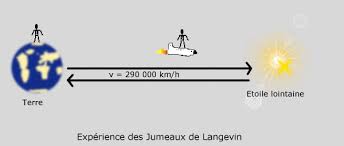
In the twin paradox, one of the twins stays on Earth while his brother makes a space journey at a speed close to the light speed and then goes back to Earth. We must then consider three Inertial references frames : the twin "at rest", the traveling twin on outward journey and the traveling twin on return journey. To date it is no longer disputed that the clocks of the two successive reference frames of the traveling twin indicate a total duration shorter than the one of the twin at rest (Multiplicity of proper times) and there is no longer a paradox. However few authors produce a demonstration of this phenomenon that is physically interpretable, with non-infinite Quadri-accelerations at the rupture points of the spatio-temporal trajectory of the traveling twin [GOU, Relativité Restreinte, p.41].
Note that the Principle of equivalence combined with the Multiplicity of proper times predicted by Restricted Relativity leads us to predict a multiplicity of proper times where there is a multiplicity of gravitational potentials. Two perfect clocks placed in places of different gravitational potentials will not record identical cumulative times. We can speak of Twin paradox bis : two twins living at different altitudes will not record the same duration.
This paradox shows that Relativity allows the journey to the future. On the other hand, the Restricted Relativity does not allow the journey to the past, which would theoretically be possible in General Relativity with gravitational field [GOU, Relativité Restreinte, p.54].
But what about the biological aging of the two twins ? Can we say that the traveling twin goes back to Earth "younger" than the sedentary twin ? Opinions are very divided :
- Poincaré never speaks of biological time and asserts that "the properties of time are only those of clocks".
- Einstein makes no claim about the time actually experienced by the inhabitants linked to a given reference frame.
- Thibault Damour, Phycisien of Relativity, asserts that even if the traveling twin goes back to Earth younger than the sedentary twin, he will not live any longer. The best image is cryogenics : instead of sending one of the twins into space, he was put in an ice block and then delivered. The proper time of the traveling twin is actually shorter than the one of the sedentary twin but he does not acquire an additional "biological time", for example the number of heartbeats.
- The effects of biological time dilation are currently unproven experimentally.
- Most astrophysicists assert that talking about biological time has no scientific meaning.
In conclusion, the extrapolation of the effects of physical time dilation to biological systems remains hypothetical and subject to debate in the scientific community.
The universe age is the time elapsed since the Big Bang. The best approximation to date is given by : 1 / H0
where H0 is the Hubble constant (See Hubble-Lemaître law),
giving an age of about 13 billion years.
The universe history, since its creation approximately 13 billion years ago, is summarized below.
| Time in years | Time reduced to one year | Event | Detail |
|---|---|---|---|
| -13 billion | January 1 | Big Bang | Birth of the universe according to the Standard Cosmological Model, with the formation of hydrogen and helium |
| -12.5 billion | February 1 | Galaxies and proto-stars | Appearance of galaxies resulting from the concentration of hydrogen atoms in an expanding universe. Within these galaxies, the first primitive stars are born, which form when clouds of very cold and dense interstellar gas collapse under the influence of gravity and cause nuclear reactions in their cores. The collapse may be due to the gravitational attraction of a nearby star, or the shock wave caused by a supernova, or the collision of two galaxies. |
| -4.6 billion | September 1 | Solar System and Earth | Appearance of our Sun within our galaxy (Milky Way). Around it, the dust aggregates into blocks, in turn forming planets including the Earth. |
| -3.5 billion | October 1 | Living organisms without a nucleus | On Earth, appearance of Prokaryotes (cells without a nucleus) including marine bacteria |
| -2.2 billion | November 1 | Living organisms with a nucleus | Appearance of the first Eukaryotes (cells with a nucleus) including brown algae |
| -1.8 billion | December 1 | Terrestrial oxygen | Appearance of free oxygen in the Earth's atmosphere |
| -600 million | December 15 | Marine organisms with shells | Appearance of shellfish and crustaceans |
| -500 million | December 19 | Fish and early vertebrates | |
| -450 million | December 20 | Land plants without flowers | |
| -400 million | December 22 | Flying insects and amphibians | |
| -300 million | December 23 | Trees and Reptiles | |
| -200 million | December 25 | Dinosaurs and mammals | |
| -150 million | December 27 | Birds and flowering plants | |
| -66 million | December 30 | Disappearance of dinosaurs | |
| -18 million | December 31 at 12:00 | Cetaceans and primates | |
| -20 million | December 31 at 2:00 p.m. | Homonidae | Appearance of the first great apes |
| -2.0 million | December 31 at 10:00 p.m. | Homo Habilis | Appearance of the first humans |
| -200 000 | December 31 at 11:56 p.m. | Homo Sapiens | Appearance of the "modern man" |
| -2 000 | December 31 at 11:59:56 p.m. | Year 0 Christian | |
| 0 | December 31 at 24:00 | Today |
Sources :
- https://fr.wikipedia.org/wiki/Calendrier_cosmique_de_Carl_Sagan
- http://www.syti.net/EvolutionStory.html
- https://www.lemonde.fr/passeurdesciences/article/2017/05/31/l-histoire-de-l-univers-condensee-en-un-an_6001909_5470970.html
- https://www4.obs-mip.fr/wp-content-omp/uploads/sites/44/2017/04/histoire_temps_univers.pdf
- https://planet-terre.ens-lyon.fr/ressource/chronologie-terre.xml
The Universe line (or spatio-temporal trajectory) of a material particle is a Space-time curve (or sequential path of events) corresponding to the history of the particle.
By definition, the universe lines of physical particles are always located inside the Light-cone at a given point (see Figure above). These are any curves of time-like type. They are Geodesics only when the material particle is not subjected to any other interaction than that induced by the gravitational field.
Any vector v of the Space-time is called :
- time-like vector when the Scalar product v.v < 0. This is the case of the vector tangent to the trajectory of a non-zero mass particle. Two events of Space-time can be connected by information going at a speed lower than light speed.
- light-like vector (or light vector or isotropic vector) when the Scalar product v.v = 0 with v ≠ 0. This is the case of the vector tangent to the trajectory of a zero mass particle (photon for example). Two events of Space-time can be connected by information going at the light speed.
- space-like vector when the Scalar product v.v > 0. This is the case of the vector neither time-like nor light-like. Two events of Space-time can not be connected by information going at the light speed.
By definition the time-like, light-like and space-like vectors are situated respectively inside, on the surface and outside the Light-cone.
A wormhole is a solution of the Einstein Equation in which the Energy-Impulse Tensor is particular, allowing to create a shortcut in Space-time.
The matter which fills the Space-time of the wormhole is a so-called "exotic" matter (not observed to date) which violates the low energy condition [GOU, General Relativity, p.259].
The authors quoted in this page are referenced in square brackets under the reference [AUTHOR Title Page].
 Last page update : July 28, 2025.